The Shopkeeper's Scale
Let me start in a small corner shop.
The shopkeeper pays rent for her shop every month. She pays it whether ten people come in or a hundred. At the end of the month she wants to know one thing: how much did each sale really cost her?

The rent alone cannot tell her. She also needs to know how many sales the rent paid for. In a busy month each sale is cheap. In a quiet month each sale is dear, even though the rent did not change. Coins go on one side of her scale, and the work they paid for goes on the other.
A machine learning service has this problem too. You rent a computer by the hour, and it answers questions with a model. In this lesson I measure how many answers one hour of a rented computer can give, on five different computers, and work out what 1,000 answers really cost.
Where This Lesson Starts
This is lesson 11 of the chapter on serving a model. Serving a model means running it as a small program that answers questions while people wait.
The model is the features chapter's model. It looks at six numbers about one customer of a real online shop, such as the days since their last order. It gives a score between 0 and 1: how likely they are to buy again in the next 30 days.
Lessons 2 to 10 measured this service on one kind of rented computer. They asked how fast it is, how it behaves when busy, and how much memory it uses. None of them asked about money.
So here is my question: what do 1,000 predictions cost? A prediction is one answer from the model, one score for one customer. To answer, I need two numbers for each computer. The first is its price per hour, which Amazon publishes. The second is how many answers it gives in that hour while still answering quickly. Nobody publishes that one, so I measured it.
The Words You Need First
Please read this slide slowly if any word is new. Each word comes with an everyday picture.
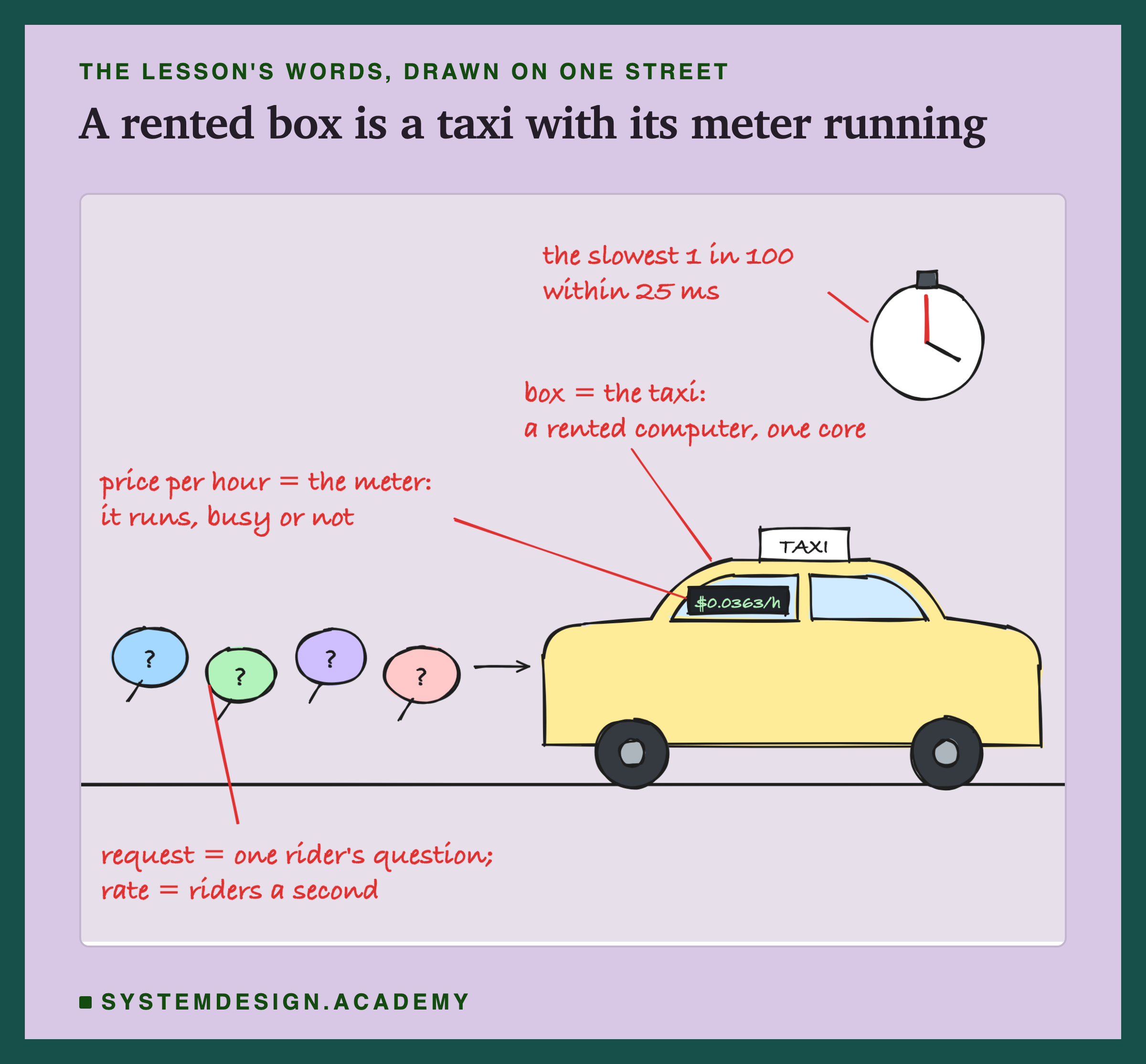
A box is my short name for a rented computer. Amazon Web Services (AWS) rents them through a service called EC2. The CPU is the chip that does a computer's work. Inside it, a core is one worker that runs one step of a program at a time. AWS rents you a share of a chip and calls one core's worth a vCPU. Every box in this lesson has one.
On-demand means renting with no promise: start the box when you like, stop it when you like, and pay a fixed price per hour. Think of a taxi meter. It runs while the taxi is yours, whether or not anyone rides.
A request is one question sent to the service, such as "score customer 12346". The rate is how many requests arrive each second.
Waiting times are in milliseconds (ms). A millisecond is a thousandth of a second, so 25 ms is a fortieth of a second. A blink of an eye takes about 100 to 400 ms, so 25 ms is a small part of one blink.
Users notice the slowest answers most, so I watch those. Line up every request's waiting time, shortest to longest. The p99 is the time that 99 out of every 100 requests beat. I will mostly say "the slowest 1 in 100", which means the same thing. My target in this lesson: the slowest 1 in 100 must answer within 25 ms.
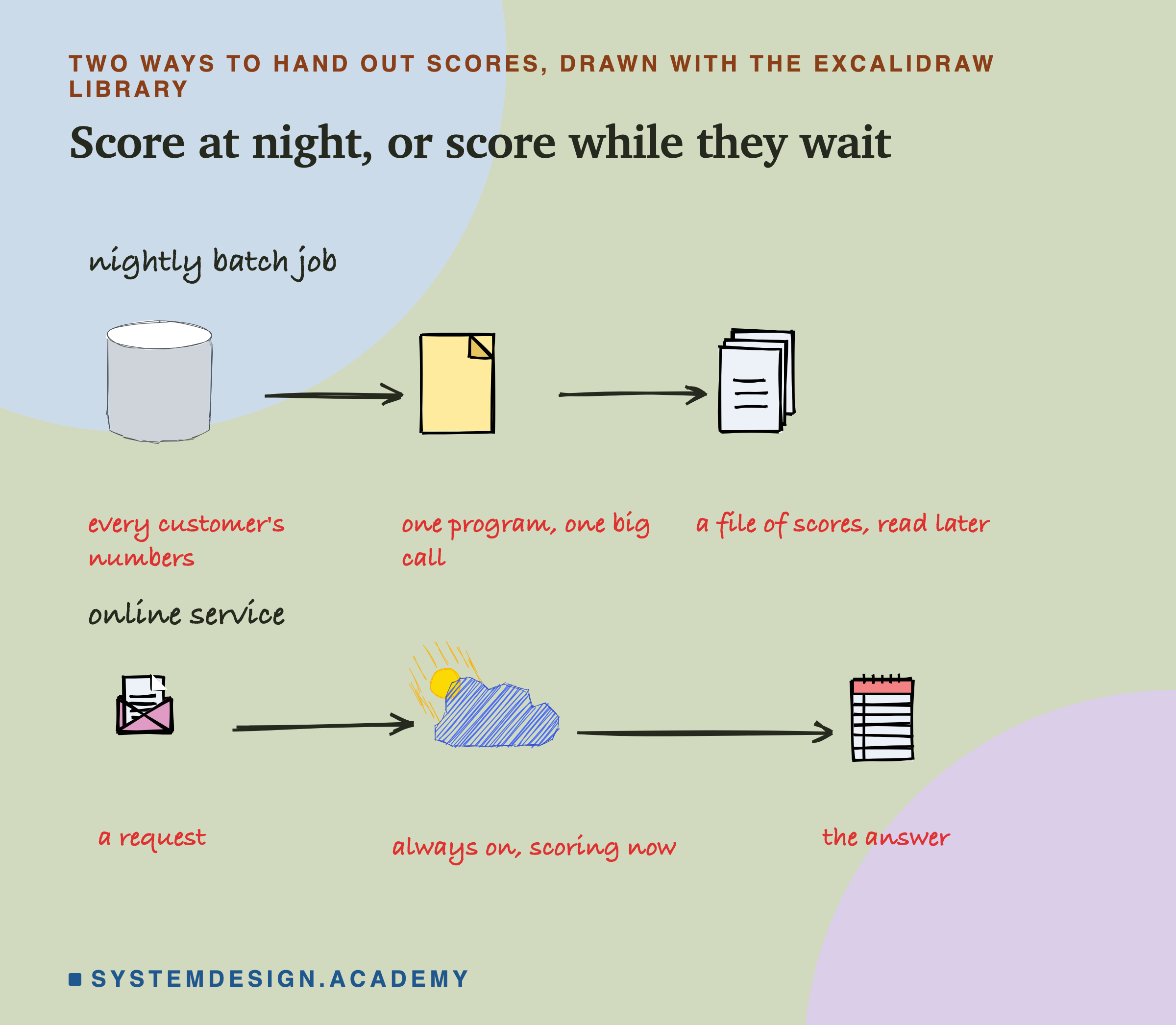
There are two ways to hand out scores. A nightly batch job scores every customer once a night and keeps the scores in a file. Online serving runs a service all the time and scores each request the moment it comes. Lesson 1 compared the two on how old the scores get. This lesson compares their price.
One more word. A call to the model is one time the program asks the model for scores. Batching means scoring several waiting requests in one call. Lesson 4 found that one call for 32 rows costs little more than one call for one row. I use its best setting: up to 32 requests in one call, and the service never waits on purpose for more to arrive. I call the other way "one by one".
The Five Machines
My AWS account may run only one core at a time, so I could rent only small one-core boxes, one after another. I picked five. Their names look like codes, so here is how to read them. The first letter says the family: "c" is AWS's family for computing work. The number is the generation. A "g" after it means AWS's own Graviton chip, and an "a" means an AMD chip. ".medium" is the smallest size, with one core. The a1.medium is an older family with its own name.
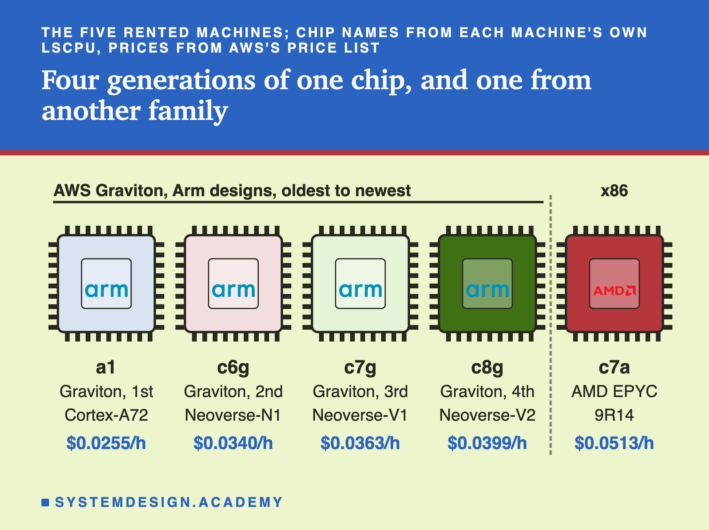
AWS makes its own chips, called Graviton. They use designs from a company called Arm, whose designs also run most phones. My four Graviton boxes cover four generations. The a1.medium has the first Graviton, the c6g.medium has Graviton2, the c7g.medium has Graviton3, and the c8g.medium has Graviton4. The c7g.medium is the box of lessons 2 to 10.
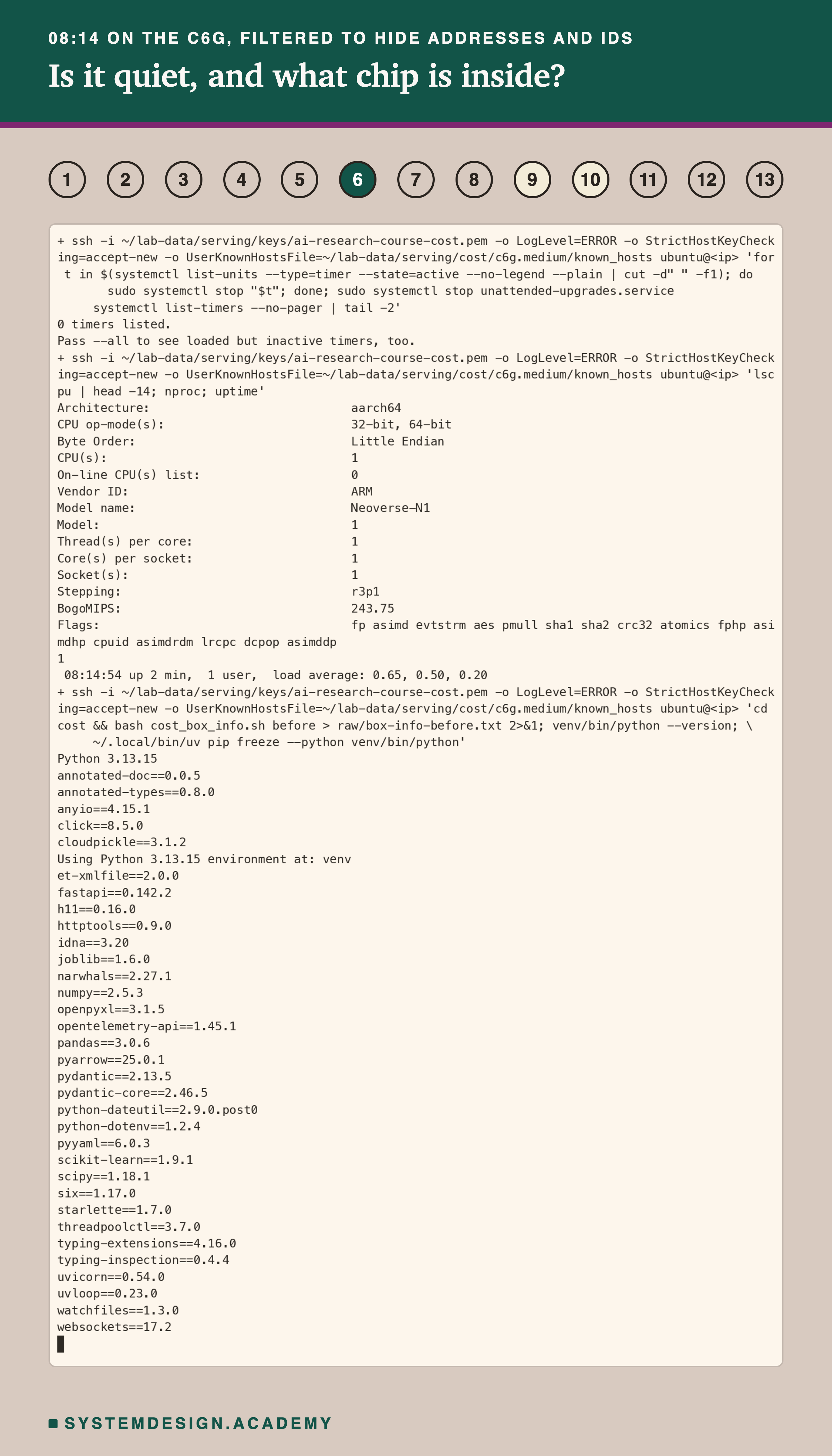
The fifth box, the c7a.medium, has an AMD EPYC chip. It is of the x86 kind, used in most Windows laptops and many servers. The two kinds understand different machine instructions, so each needs its own copy of Python. A package is a ready-made box of code, such as numpy. The command pip freeze prints every installed package and its version, and its list was identical on all five boxes.
Each box reported its own core design through lscpu, a command that describes the processor. The names in the picture, such as Neoverse-N1, are Arm's and AMD's names for those designs.
Every box has 2 GiB of memory, about two billion bytes; one byte holds one letter. None is burstable, a kind of box whose speed drops after a busy spell. All ran Linux, the system that runs most servers, in us-east-1, Amazon's group of data centres in Virginia, USA. Prices per hour come from AWS's own price list, read on 2026-10-11.
The Headline: Read the Unit Price
A good supermarket shows two prices on a shelf label: the price of the packet, and the unit price, such as the price per kilogram. The unit price tells you which packet is the better deal. Here are my five boxes as shelf labels.
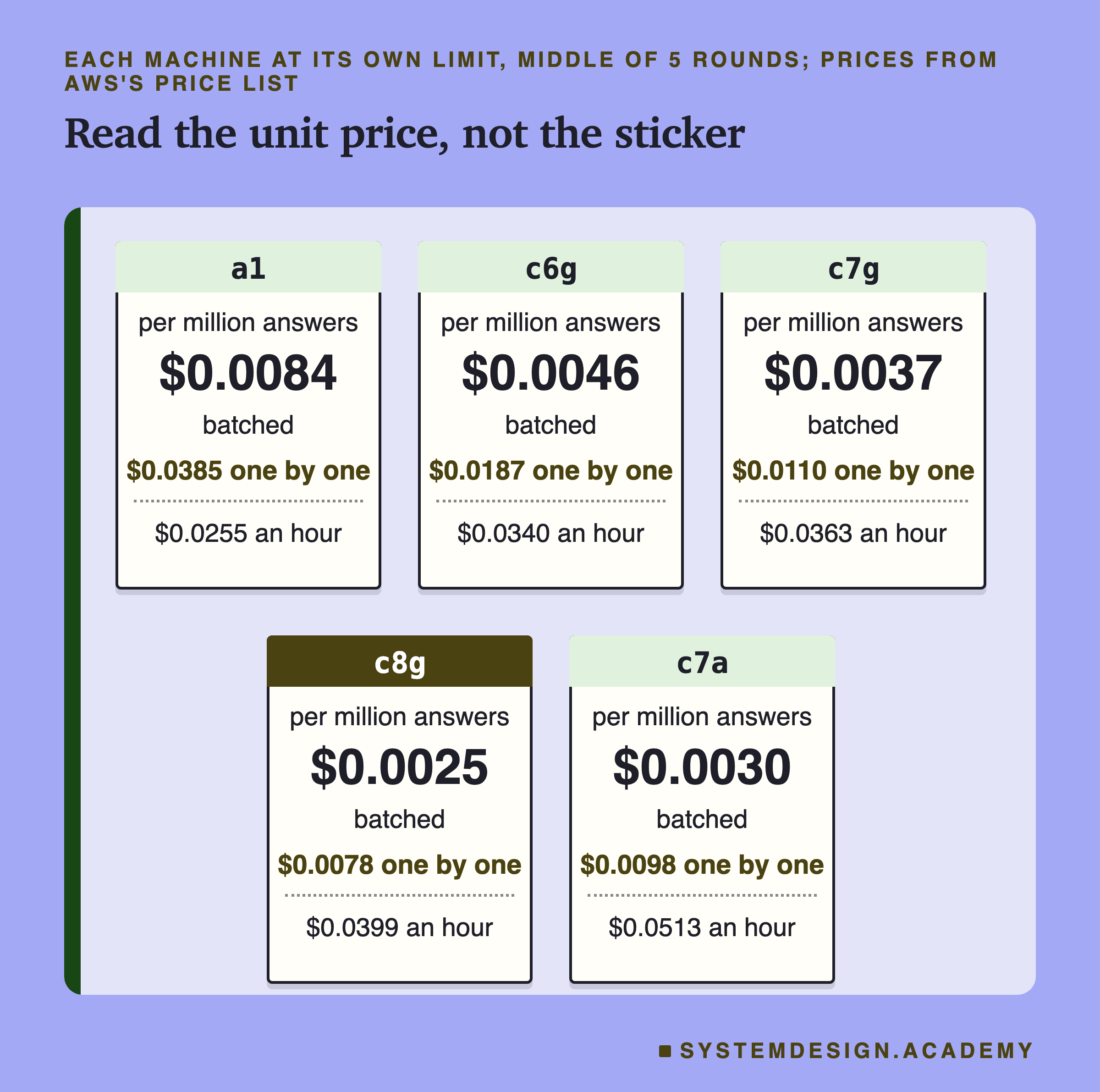
Each label's big number is the cost of a million answers with batching, with the box at its own limit. A box's limit is the most requests a second that still kept the slowest 1 in 100 under 25 ms. Under it is the cost one by one, and at the bottom the sticker price per hour. The numbers are the middle of 5 rounds of testing.
The a1.medium has the cheapest sticker, $0.0255 an hour, and the dearest unit price. One by one, a million answers on it cost $0.0385, five times the c8g.medium's $0.0078. It answered too slowly to make its low price pay.
The newest chip won. The c8g.medium was cheapest per answer both ways, and batched it gave a million answers for $0.0025, about a quarter of a cent.
Batching mattered on every box. It cut the cost per answer to between 22% and 34% of the one-by-one cost, because each hour gave 3.0 to 4.6 times as many answers.
Two warnings come with these labels. First, my test program shared each box's one core with the service: it took 4 to 9% of the core one by one, and 13 to 19% batched. So every rate here is a little low, the batched ones more. Second, the labels assume each box is busy at its limit every second. A real service is quiet for much of the day, and the meter still runs. Later slides price both of those.
How the Lab Was Built
Before any run, I wrote the lab's plan at the top of its program file, scripts/labs/serving/cost_per_prediction.py. That note at the top of a Python file is called a docstring. It names every setting and the rule for "clearly different", and it lists twelve guesses, written first so they could be checked later and could be wrong.
The service is lesson 4's, copied unchanged, with lesson 2's model and lesson 2's small database of customer numbers. It runs as one program with one thread, one line of work inside a program, which lesson 5 found fastest on one core. I ran it two ways and call each way an arm, like one recipe in a cooking test: one by one, and batched.
A tester is a program that pretends to be many users sending questions. Mine is lesson 7's honest tester. It plans every request's arrival time before the run, at random, like customers walking into a shop. Then it sends each request at its planned time, even if earlier answers are late, and times each answer from the planned arrival. Time spent waiting in a queue therefore counts. Each counted run lasted 12 seconds.
To find a box's limit, I climbed. A quick first climb, which I call the scout, found roughly where the limit was. Then I fixed ten rates around it, each about 6% higher than the last, like the steps of a staircase. A run passed if its slowest 1 in 100 took at most 25 ms and the service kept up with the arrivals.
Each box ran 5 rounds. A round tries every rate of both arms once, plus one nightly batch job. Each round runs in a new random order, so the time of day could not favour one arm. In each round, an arm's max rate is the highest rate that passed with every lower rate passing too. When I say "middle round", I mean the middle of the five values.
Here is my rule for calling two arms on one box clearly different. One arm beat the other in all 5 rounds, and even its worst round beat the other's best. Boxes ran at different hours, so for two boxes I only ask that their two sets of 5 values do not overlap at all. Anything else is .
One Machine's Day on Its Own Clock
Here is the first box's day, the c6g.medium, as one numbered sequence. The numbers on the arrows match the numbers on the recordings that follow.
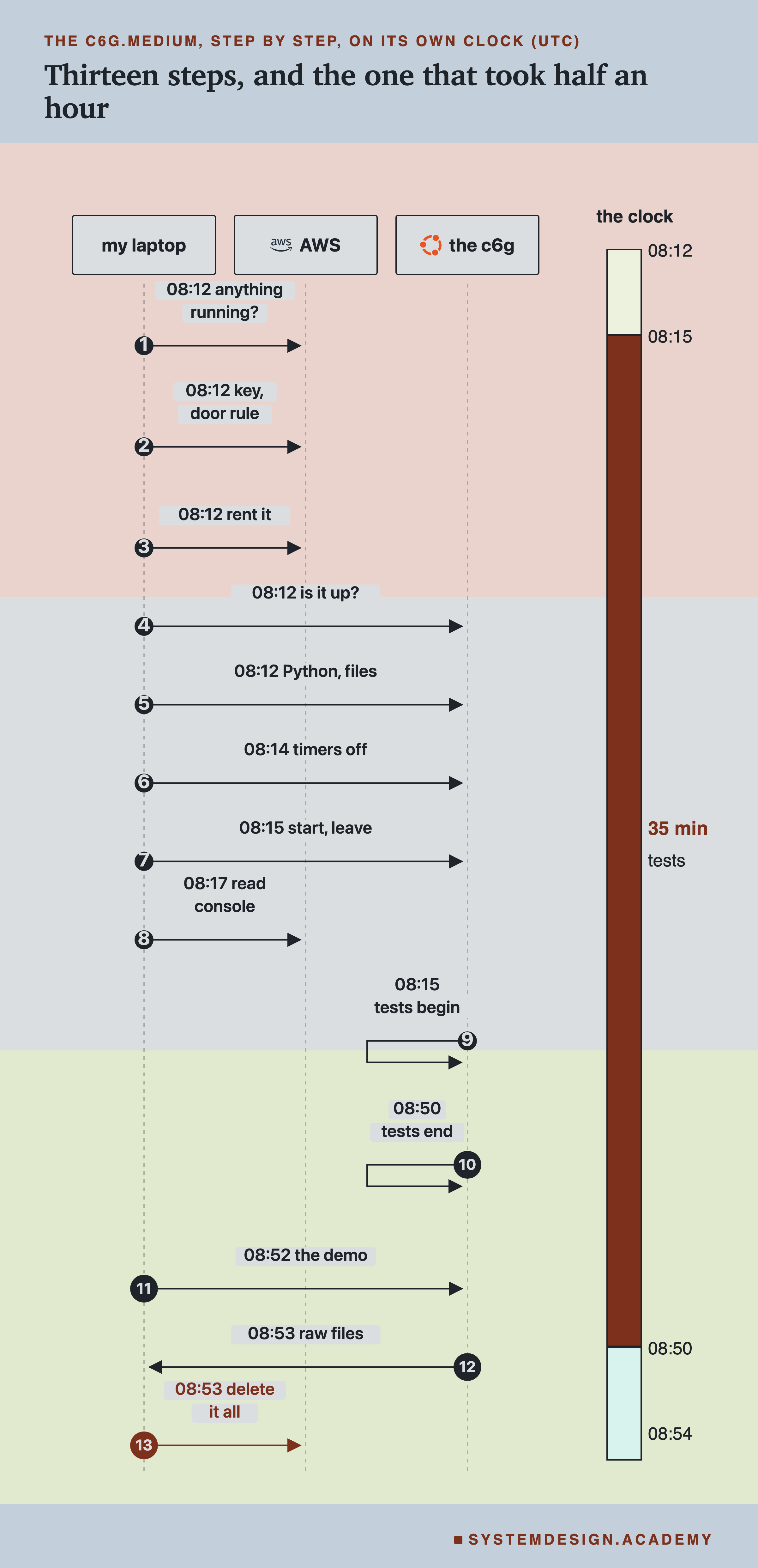
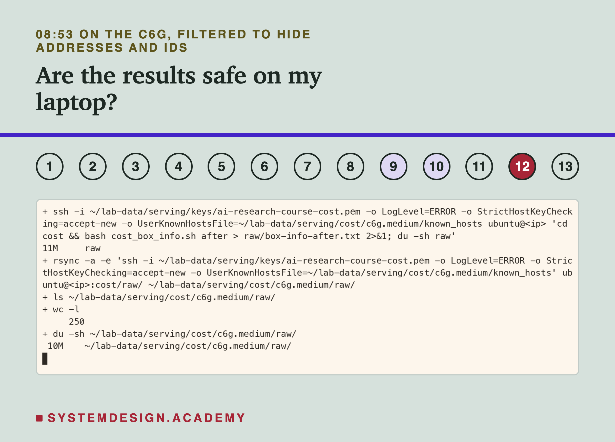
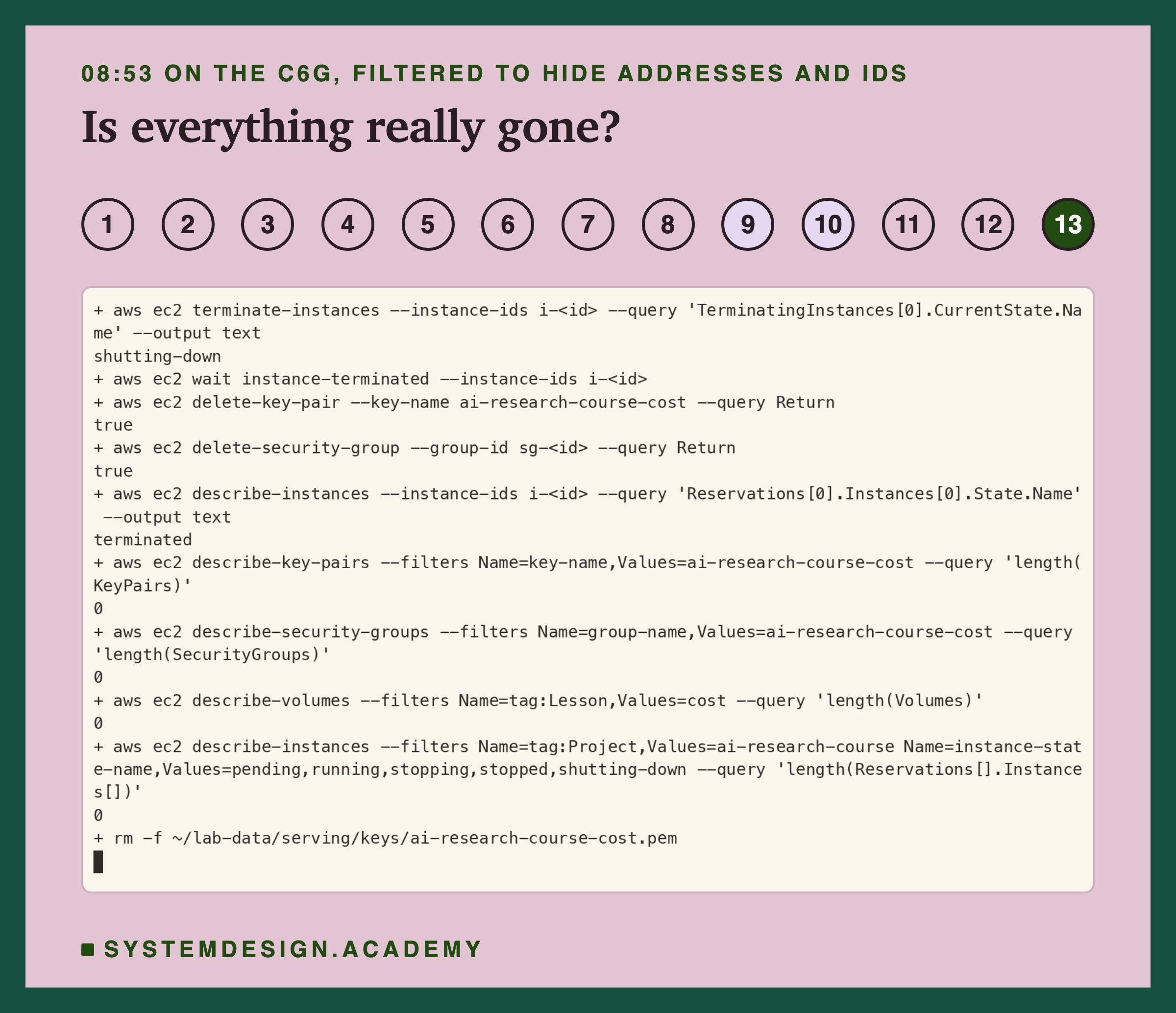
Steps 1 to 7 rent the box, set it up and start the schedule, a program on the box that runs every test in order, by itself. Step 8 is how I watched without logging in. Arrows 9 and 10 are the half hour of tests, the long dark part of the clock bar. Steps 11 to 13 came after: the student demo, the copy of the results to my laptop, and the deletion of everything. The whole day took 42 minutes.
The other four boxes went through steps 1 to 10, 12 and 13 in that order, driven by a script. On them, step 8 was a status command that reads that console, and step 11, the demo, did not run.
Build the Lab Machine Yourself
The rented boxes are part of the lab, so I show every step. You can rent this kind of box and run my schedule.
Every recording comes from the first box, the c6g.medium, the box that measured its own numbers. I did not record the other four boxes. The script that drove them is at the end of this slide.
What you need first. An AWS account, and the AWS command line tool (aws) set up with your keys. You also need four small programs you type commands into. ssh logs in to another computer, scp and rsync copy files to and from it, and curl downloads a web page. You also need lesson 2's model and data files in ~/lab-data/serving/lat, which lesson 2's lab makes.
All the steps live in one file, scripts/labs/serving/cost_files/cost_aws_steps.sh. You run it from the scripts/labs/serving folder, one step at a time, such as TYPE=c7g.medium bash cost_files/cost_aws_steps.sh check, then access, and so on. Every code block below is copied word for word from that file.
If you paste the blocks by hand, set TYPE first, such as TYPE=c6g.medium, then run these lines from the scripts/labs/serving folder. All of them come from the file, except : the file works out that folder from its own location, which a pasted line cannot do.
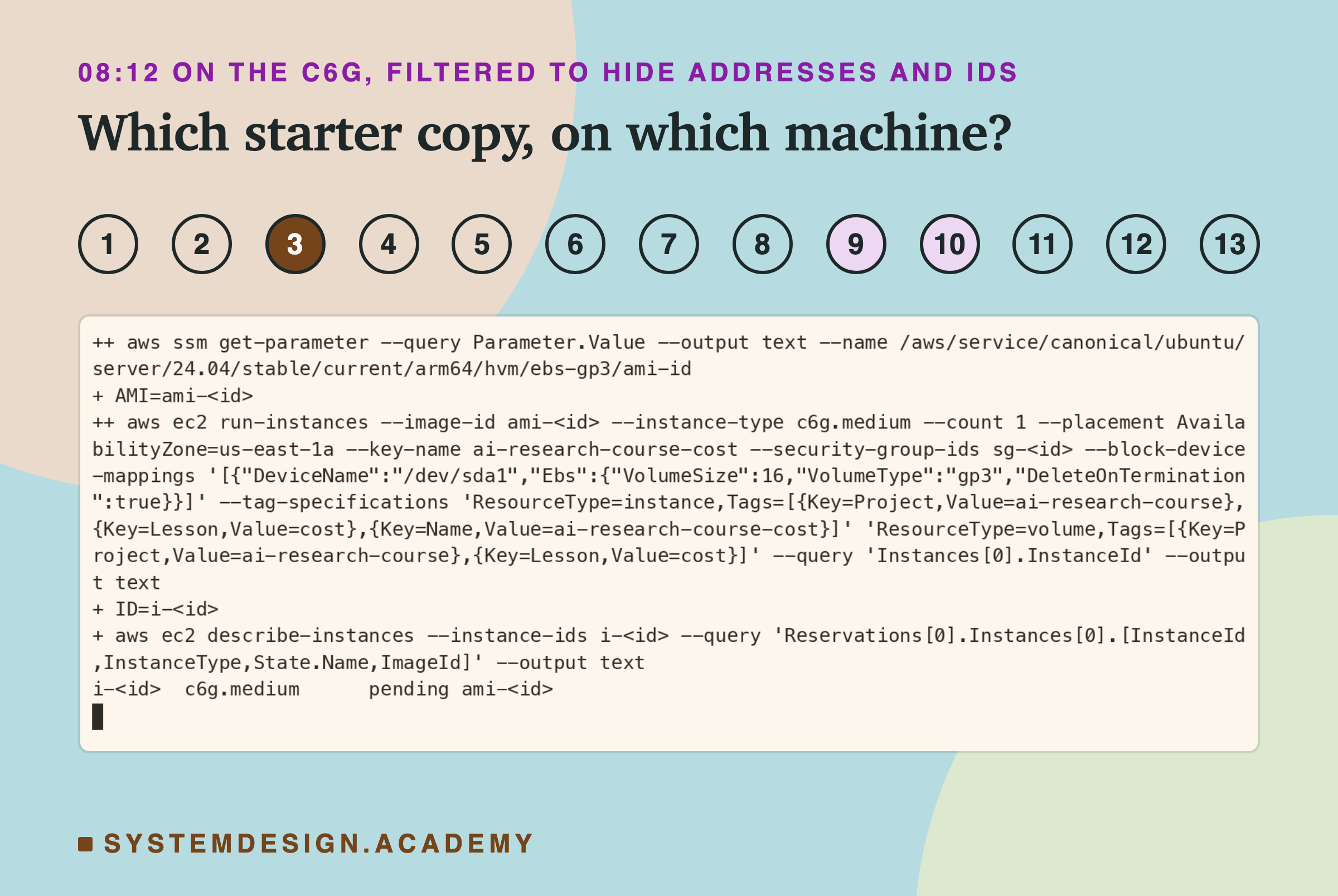
Steps 1 to 3: Is the Account Free? Lock the Door, Rent the Machine
Step 1: is any other box running? My account allows one core at a time, and another project may be using it. So the first command counts every box in the account that is starting, running or stopping. It must print 0.
Step 2: a key and a locked door. A key pair is how you prove to the box that you may come in. AWS keeps one half, and you keep the other half in a file only you can read. A security group is a door rule. A port is a numbered door on a computer, and SSH, the secure remote login, uses door 22. My rule opens only door 22, and only to my own address. Both get tags, small labels that say which project and lesson they belong to.
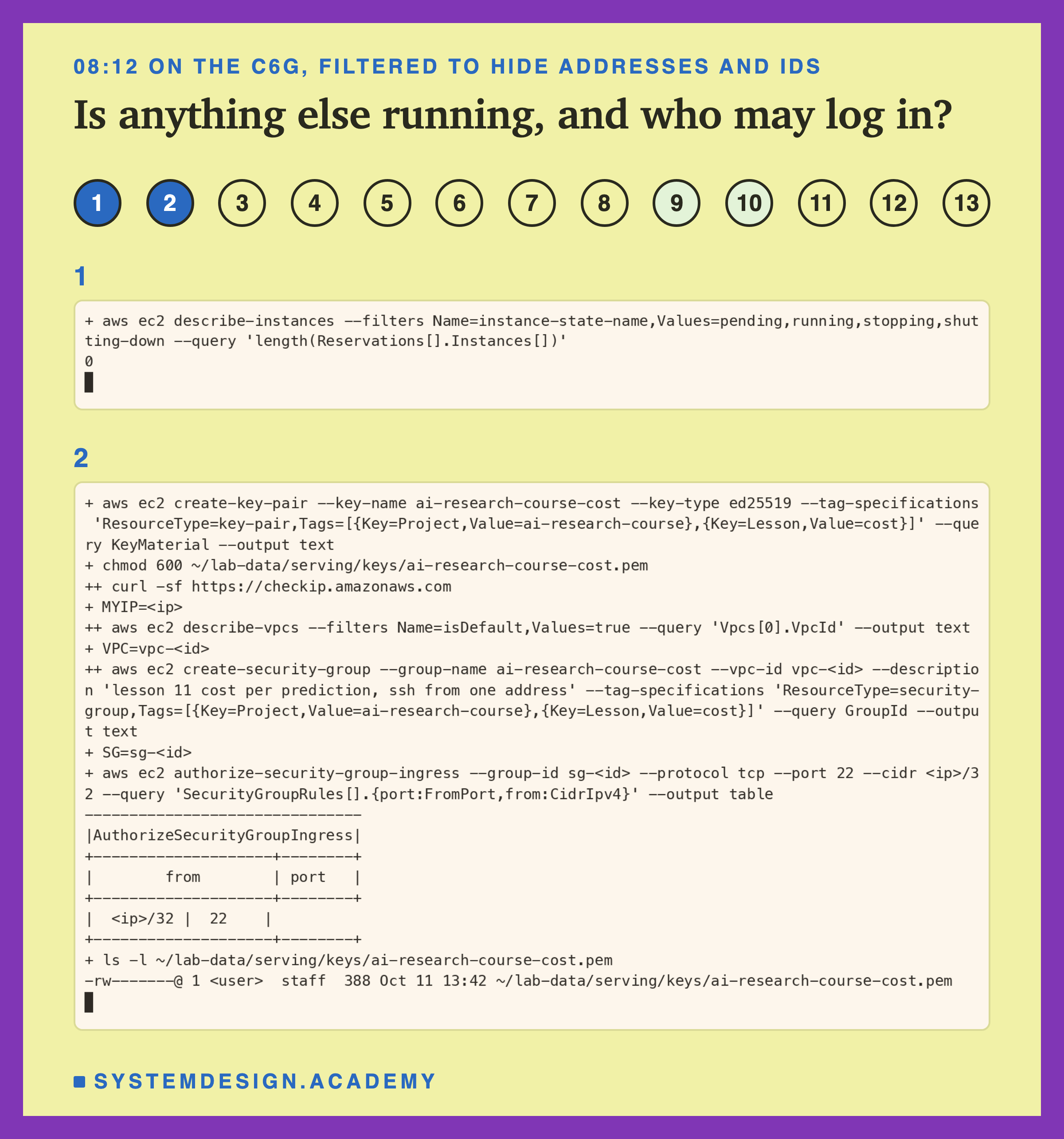
Step 1 printed 0, so the account was free. In step 2 the key went straight into its file and was never printed. This is step 1's command:
  aws ec2 describe-instances \
    --filters "Name=instance-state-name,Values=pending,running,stopping,shutting-down" \
    --query "length(Reservations[].Instances[])"
These are step 2's commands:
  aws ec2 create-key-pair --key-name ai-research-course-cost --key-type ed25519 \
    --tag-specifications "ResourceType=key-pair,Tags=[{Key=Project,Value=ai-research-course},{Key=Lesson,Value=cost}]" \
    --query KeyMaterial --output text > ~/lab-data/serving/keys/ai-research-course-cost.pem
  chmod 600 ~/lab-data/serving/keys/ai-research-course-cost.pem
  MYIP=$(curl -sf https://checkip.amazonaws.com)
  VPC=$(aws ec2 describe-vpcs --filters Name=isDefault,Values=true --query "Vpcs[0].VpcId" --output text)
  SG=$(aws ec2 create-security-group --group-name ai-research-course-cost --vpc-id "$VPC" \
    --description "lesson 11 cost per prediction, ssh from one address" \
    --tag-specifications "ResourceType=security-group,Tags=[{Key=Project,Value=ai-research-course},{Key=Lesson,Value=cost}]" \
    --query GroupId --output text)
  aws ec2 authorize-security-group-ingress --group-id "$SG" --protocol tcp --port 22 --cidr "$MYIP/32" \
    --query "SecurityGroupRules[].{port:FromPort,from:CidrIpv4}" --output table
  ls -l ~/lab-data/serving/keys/ai-research-course-cost.pem
  echo "$SG" > "$STATE/sg"
Steps 4 to 6: Wait, Set Up, Look
Step 4: wait until it runs. The AWS tool waits until the box is running. Then the script reads its public address into IP and tries SSH every five seconds until the box answers. It writes down the moment SSH first worked, because the nightly job's bill needs to know how long a box takes to start.
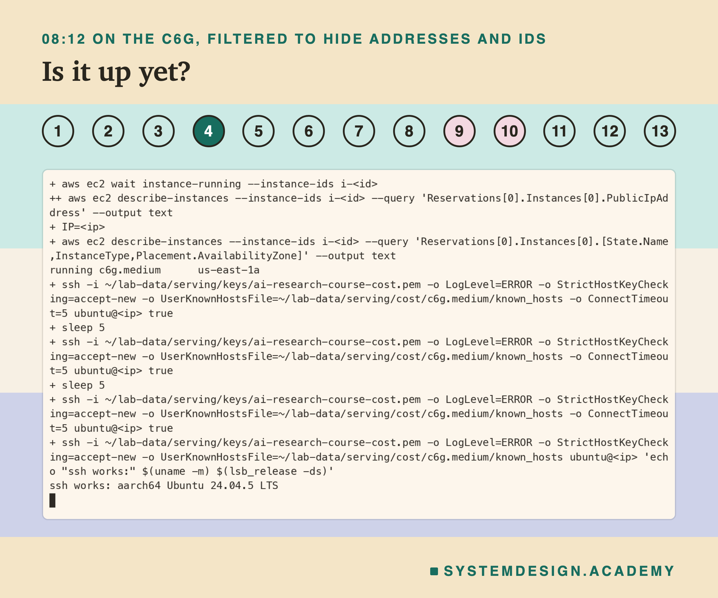
SSH failed twice while the box was still starting, then worked. "aarch64" is Linux's name for an Arm chip. These are the commands:
  aws ec2 wait instance-running --instance-ids "$ID"
  IP=$(aws ec2 describe-instances --instance-ids "$ID" \
    --query "Reservations[0].Instances[0].PublicIpAddress" --output text)
  aws ec2 describe-instances --instance-ids "$ID" \
    --query "Reservations[0].Instances[0].[State.Name,InstanceType,Placement.AvailabilityZone]" --output text
  until ssh -i ~/lab-data/serving/keys/ai-research-course-cost.pem "${SSHO[@]}" -o ConnectTimeout=5 \
    ubuntu@"$IP" true 2>/dev/null; do sleep 5; done
  ssh -i ~/lab-data/serving/keys/ai-research-course-cost.pem "${SSHO[@]}" ubuntu@"$IP" \
    'echo "ssh works:" $(uname -m) $(lsb_release -ds)'
  date -u +%Y-%m-%dT%H:%M:%S+00:00 > "$STATE/ssh_ready"
  echo "$IP" > "$STATE/ip"
  aws ec2 describe-instances --instance-ids "$ID" --query "Reservations[0].Instances[0].LaunchTime" \
    --output text > "$STATE/launched"
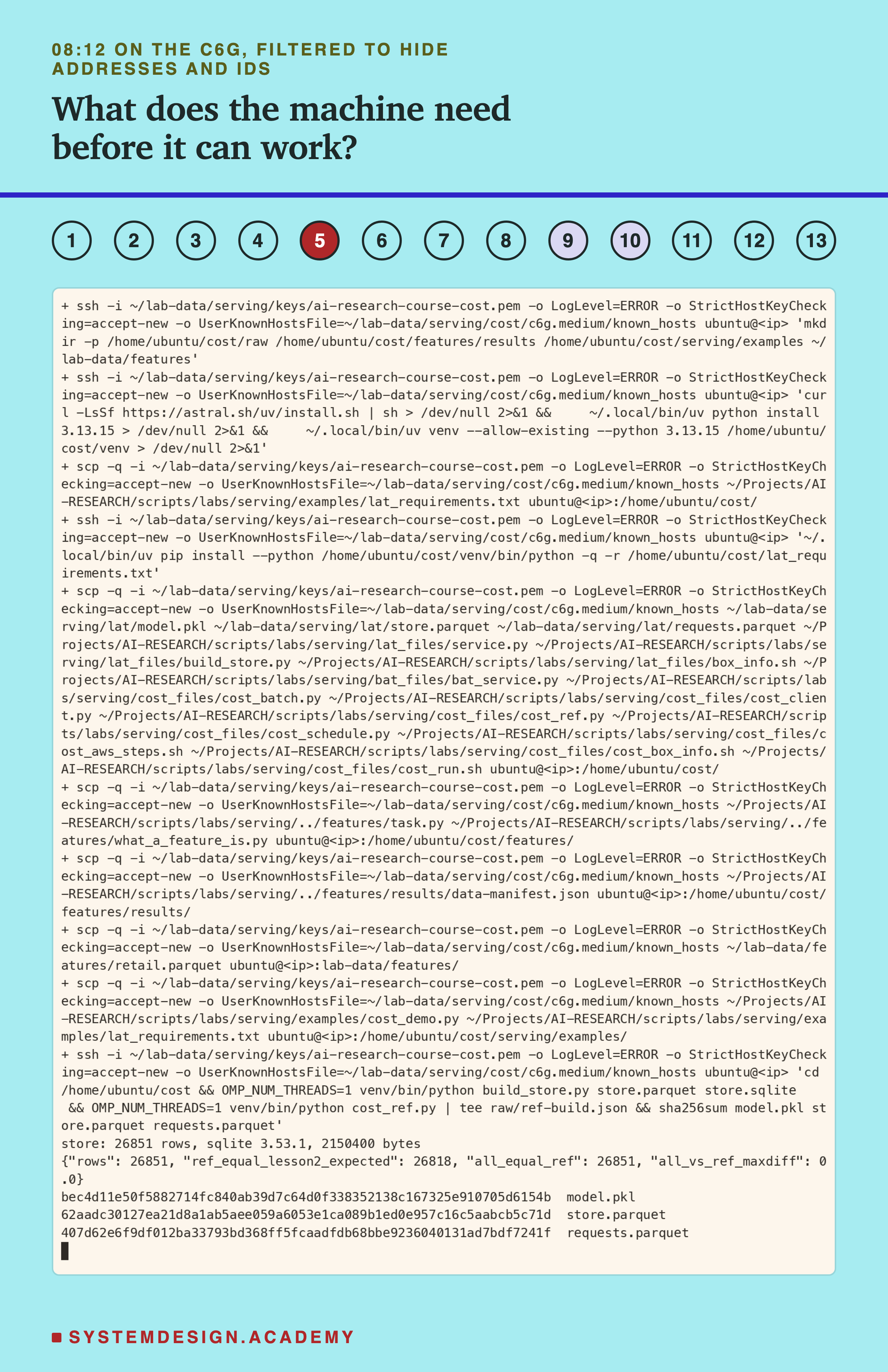
Step 5: Python, the model and the lab files. The box gets Python 3.13.15 and the library versions of lessons 2 to 10, through uv, a fast installer for Python. A venv is a private toolbox folder for one project's Python, with exact versions written down. Then scp sends lesson 2's model and data, lesson 4's service and this lesson's files.
Last, the box builds its small database and scores all 26,851 request rows once, one at a time. Those are its reference scores: the box's own score for every row, kept to check every later answer against. Then it prints three fingerprints. A fingerprint is a long code worked out from a file's bytes; it changes if even one byte changes.
Steps 7, 8 and 11 to 13: Start, Watch, Demo, Bring It Home, Delete
Step 7: start the schedule, then leave. The schedule starts in the background with setsid nohup, a command that keeps a program running after I log out. Nobody logs in again until it ends.
Step 8: watch without touching. After every run, the schedule writes one progress line to the box's serial console, a log that AWS keeps for the box. You can read it through AWS without logging in.
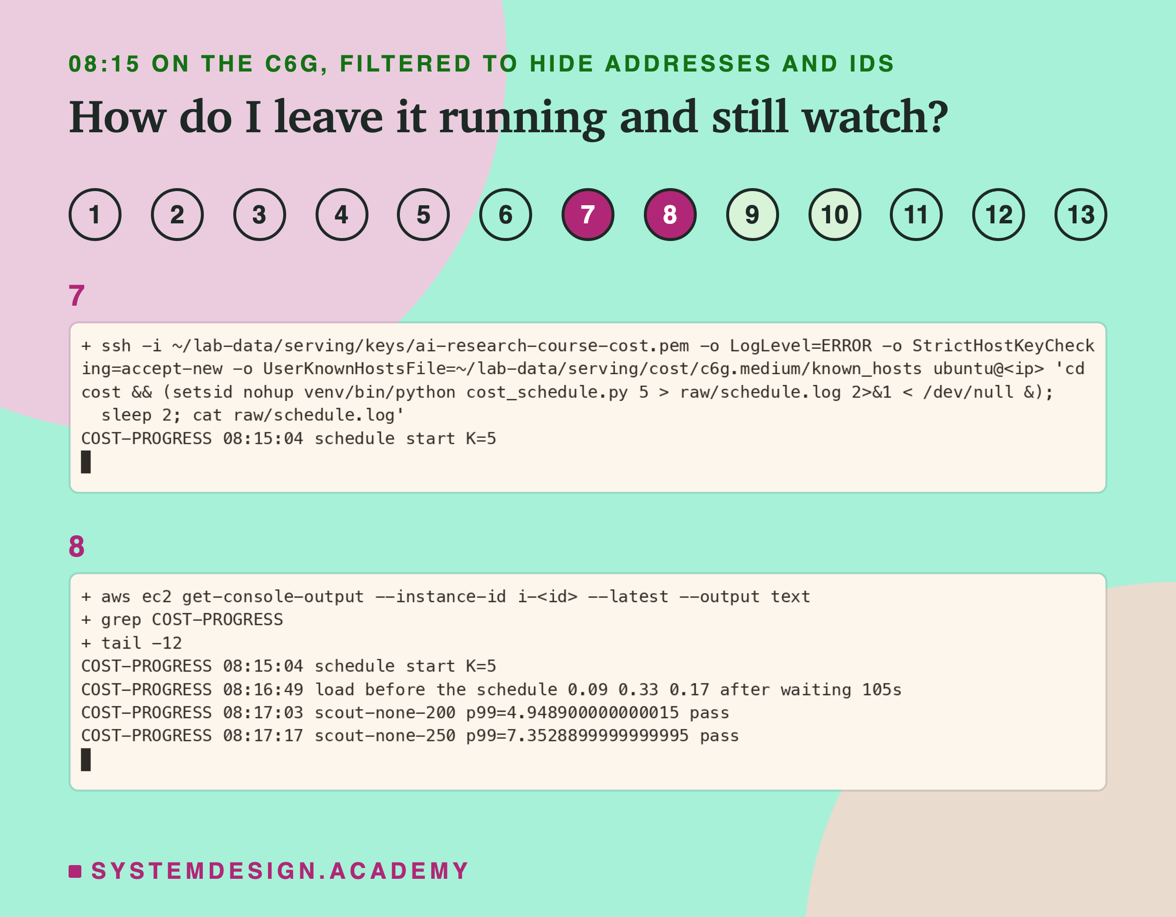
The number 5 is the count of rounds. These are the two commands:
  ssh -i ~/lab-data/serving/keys/ai-research-course-cost.pem "${SSHO[@]}" ubuntu@"$IP" \
    "cd cost && (setsid nohup venv/bin/python cost_schedule.py $K > raw/schedule.log 2>&1 < /dev/null &); \
     sleep 2; cat raw/schedule.log"
aws ec2 get-console-output --instance-id "$ID" --latest --output text | grep COST-PROGRESS | tail -12
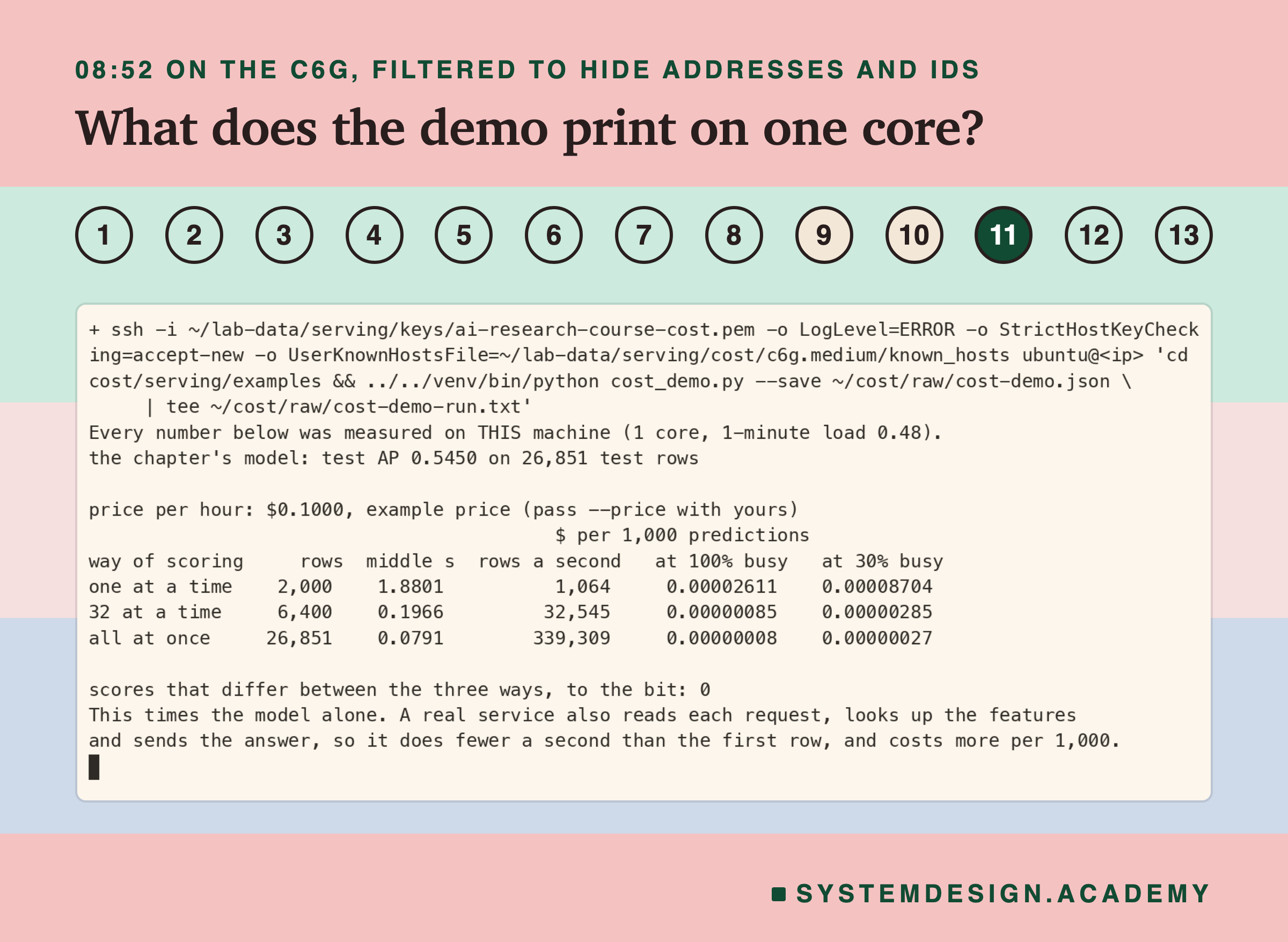
Step 11: the student demo, on that box. After the schedule, I ran the demo you will meet later, so you can see what it prints on one core.
The Lab's Report, Running
This is a real recording of the report script, cost_report.py. It ran on my laptop, but it measures nothing. It reads the raw files the five boxes wrote and does all the arithmetic again with its own code.
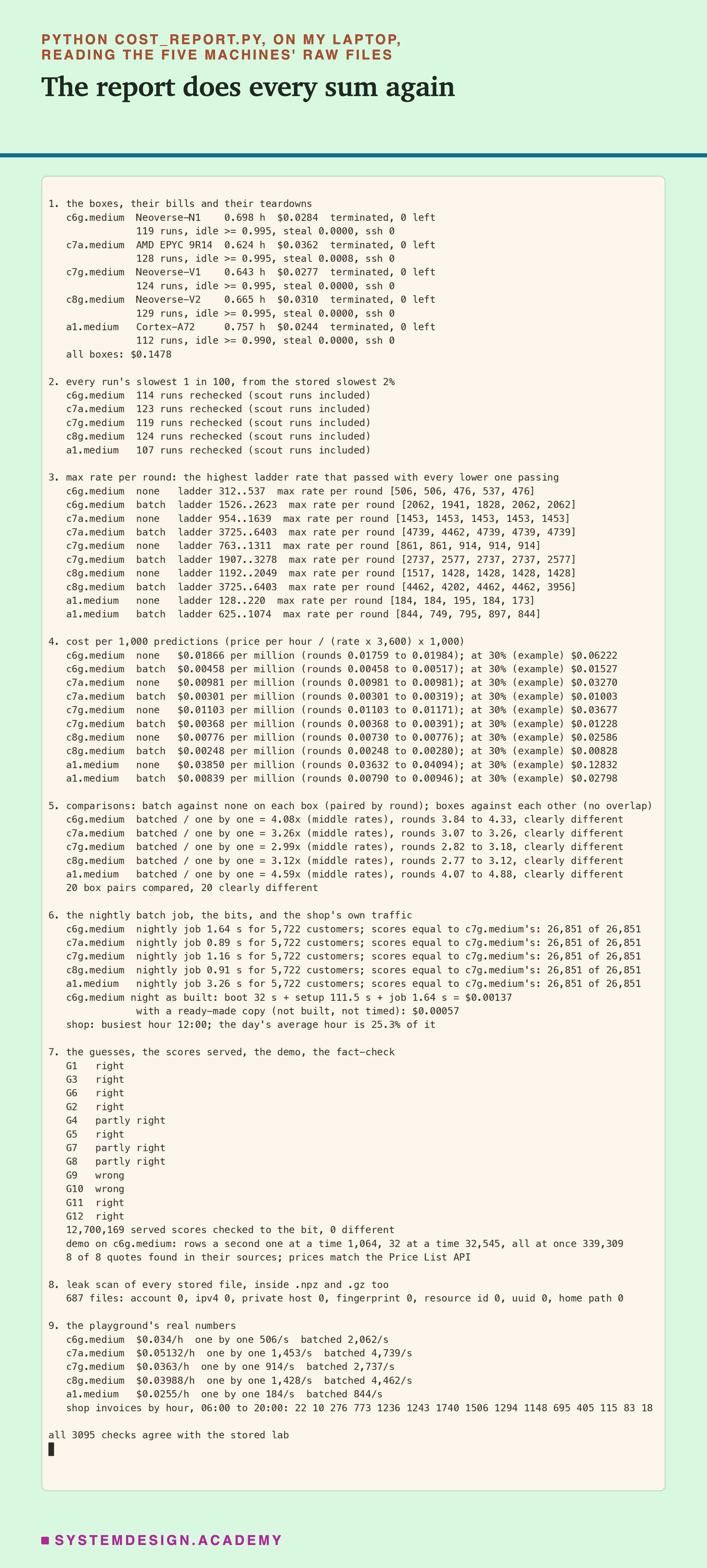
The report does not import the lab. For every run, it works out the slowest 1 in 100 again from the stored slowest 2% of waits. It also redoes each pass or fail, each max rate, each cost and each verdict, then compares every one with the lab's results file. If any number disagreed, it would stop with an error. I tried that: I changed one stored cost by a millionth of itself, and the report printed "MISMATCHES" and stopped. Then I put the file back.
Section 8 scans every stored file, even inside the packed .npz number files and the terminal recordings. It looks for my account number, IP addresses, host names, AWS ids, secret-looking codes such as key fingerprints and request ids, and my home folder. It found none of any kind.
The Meter's Sum
Every cost in this lesson comes from one small sum. Let me work it through once, slowly, with the chapter's own box, the c7g.medium, scoring one by one.
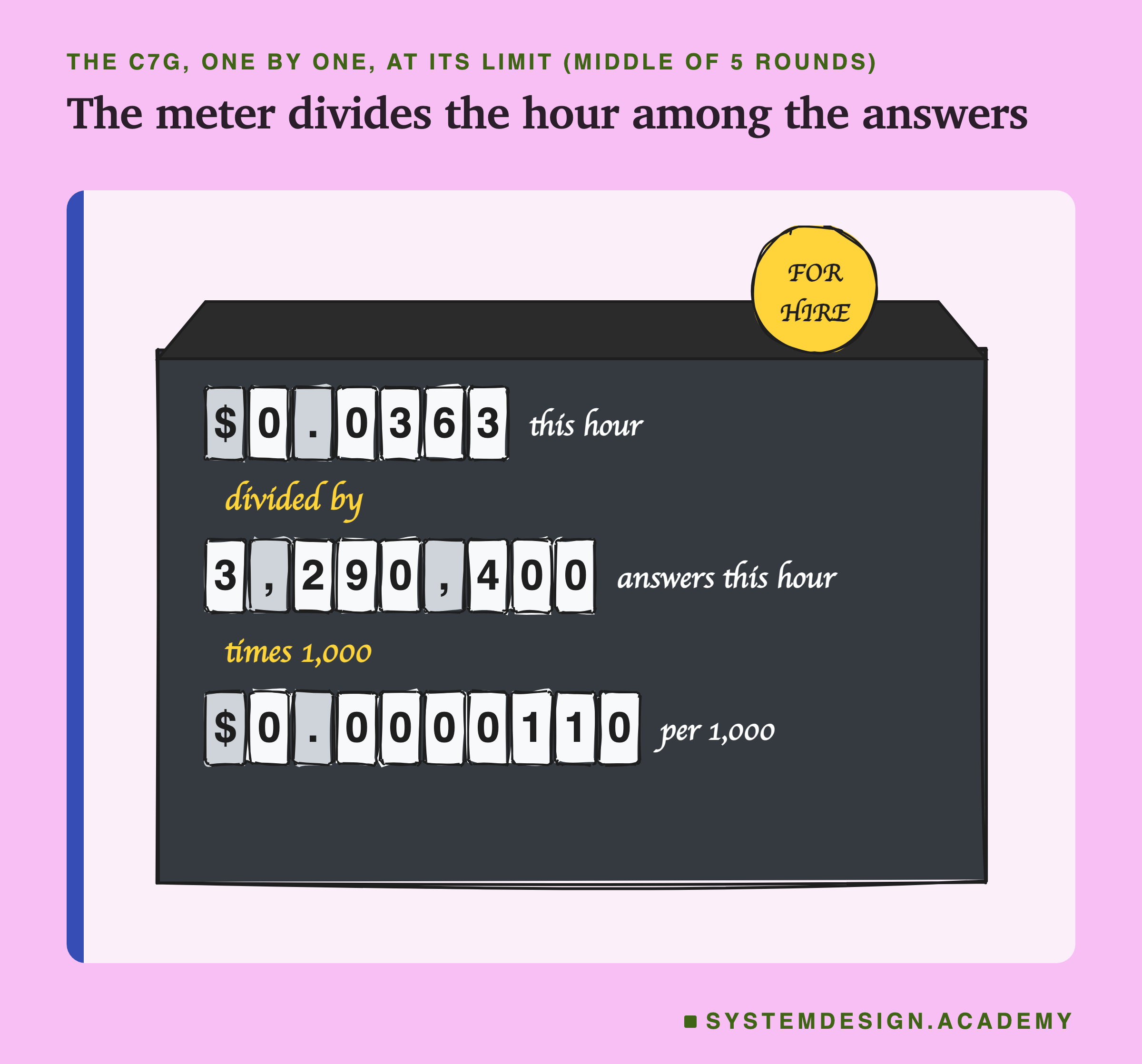
The box costs $0.0363 an hour. In the middle round it kept its slowest 1 in 100 under 25 ms at up to 914 requests a second. An hour has 3,600 seconds, so that is 3,290,400 answers in one hour. Divide the price by the answers and multiply by 1,000: $0.0000110 for 1,000 answers.
That number is too small to read easily, so from here on I give the cost of a million answers. For this box, one by one, a million answers cost $0.0110, about one cent.
Read this as the best case. The sum assumes the box is busy at its limit every second of the hour, and a meter keeps running when nobody rides.
Climbing the Staircase
How did I find "up to 914 a second"? The picture shows a search like it, for the c7g.medium with batching, one step at a time.
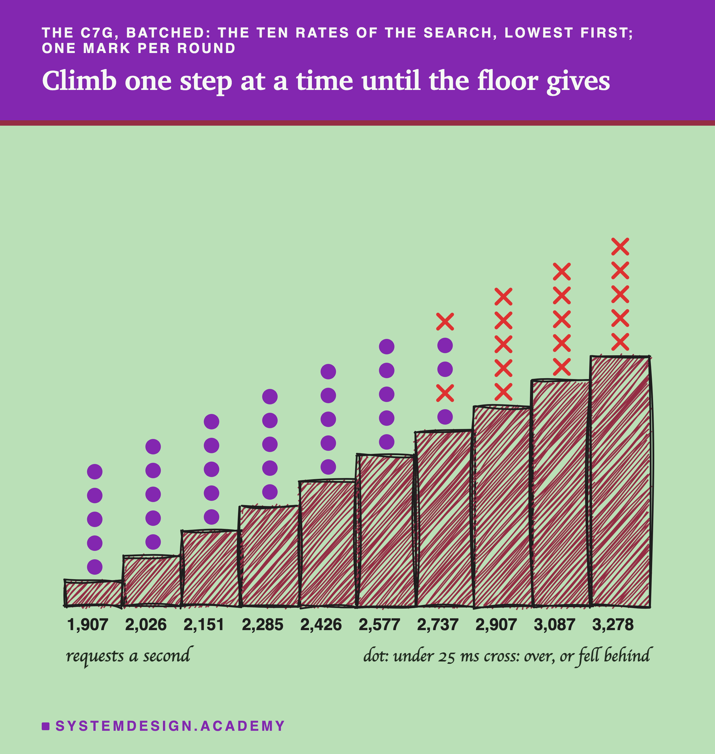
Each step is one rate, lowest on the left. On each step, each round left one mark. A dot means the slowest 1 in 100 stayed under 25 ms and the service kept up; a cross means it did not. The scout had placed the staircase around the limit, so the low steps passed every time and the high steps never did.
The limit moved a little between rounds. In 3 rounds the highest passing step was 2,737 a second, and in the other 2 it was 2,577, the step below. Steps are about 6% apart, so that is as finely as this search can see: a real limit anywhere between two steps lands on the lower one.
Why does the floor give way so suddenly? Below the limit, requests sometimes arrive a little faster than average, and the service catches up afterwards. Above it, the service cannot catch up; the line of waiting requests grows, and every later request waits behind it. On the limit's own step, the slowest 1 in 100 took 13 to 16 ms. On the next step up, only about 6% faster, it took 63 to 505 ms.
Every Machine Has a Knee
Now all five boxes, one by one.
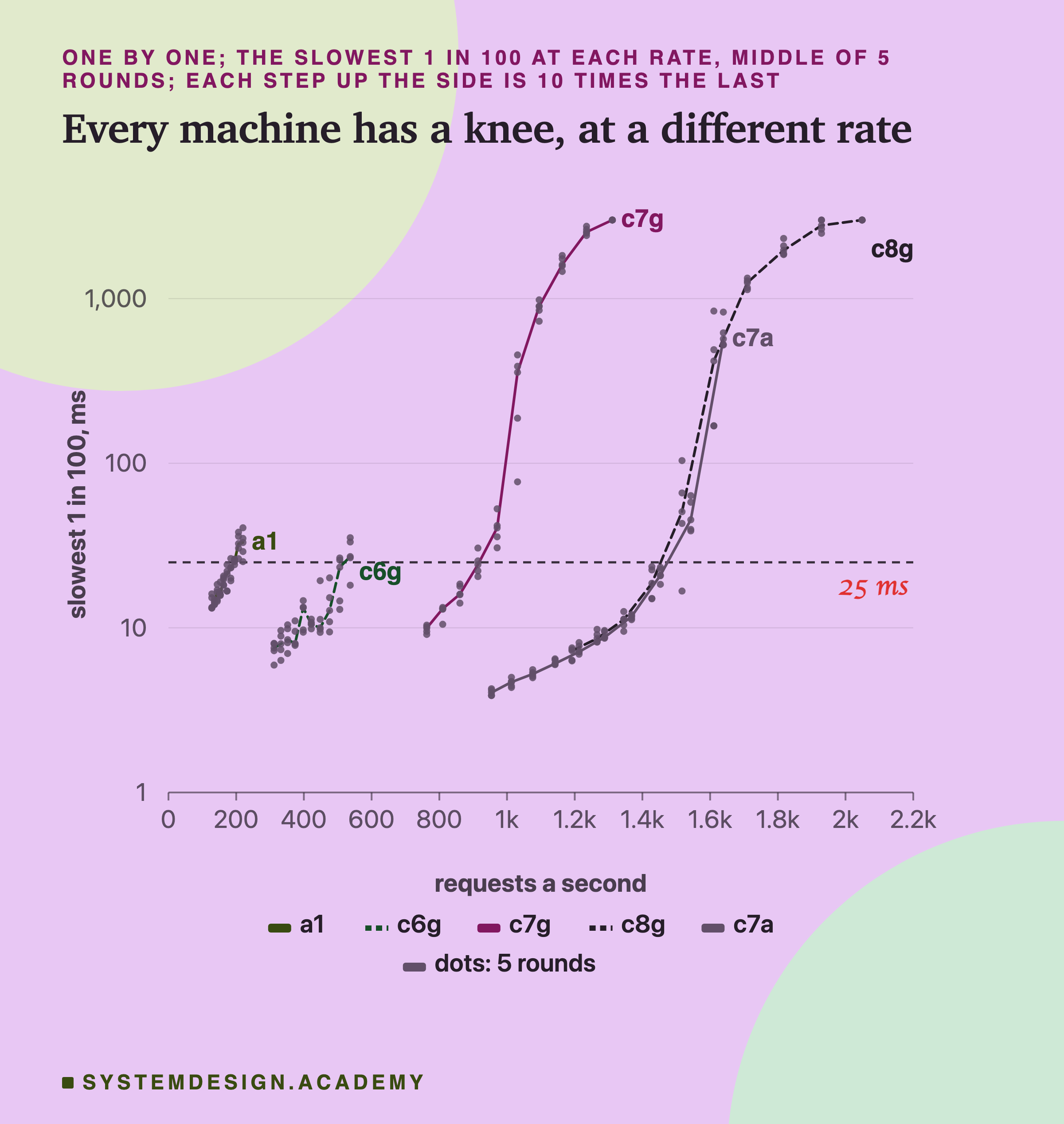
Every line has one shape. It stays low and nearly flat, then bends up sharply and crosses 25 ms. I call the bend the knee. Only where it happens differs, from about 184 a second on the a1.medium to about 1,450 on the c8g.medium and c7a.medium.
The c7g.medium's knee sat at 861, 861, 914, 914 and 914 a second over the 5 rounds. Lesson 4 measured this service on a different c7g.medium, rented on another day: there 879 a second passed and 1,098 fell behind. The two boxes agree.
Batching Multiplied the Rate
Next, the two arms side by side.
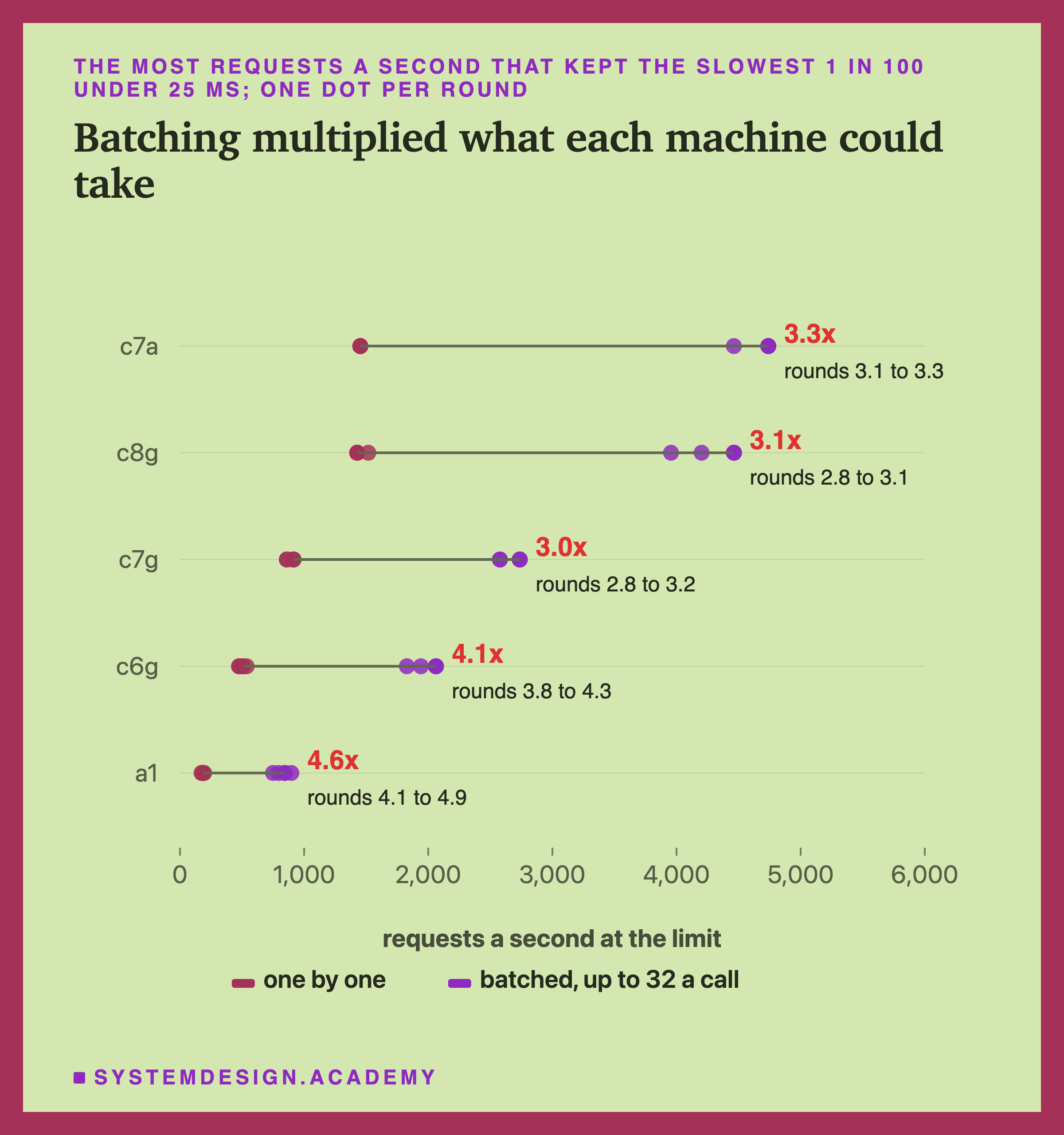
The red number is the middle batched rate divided by the middle one-by-one rate, so you can check it from the two dots it sits between. It was 4.6 on the a1.medium, 4.1 on the c6g.medium, 3.0 on the c7g.medium, 3.1 on the c8g.medium and 3.3 on the c7a.medium. Under it is the range of the five per-round ratios. On every box, batching won in all 5 rounds and the two sets of 5 did not overlap, so it is clearly different everywhere.
Why so much? Near the limit, requests pile up, so each call to the model took a handful of them at once. A call's fixed cost was shared.
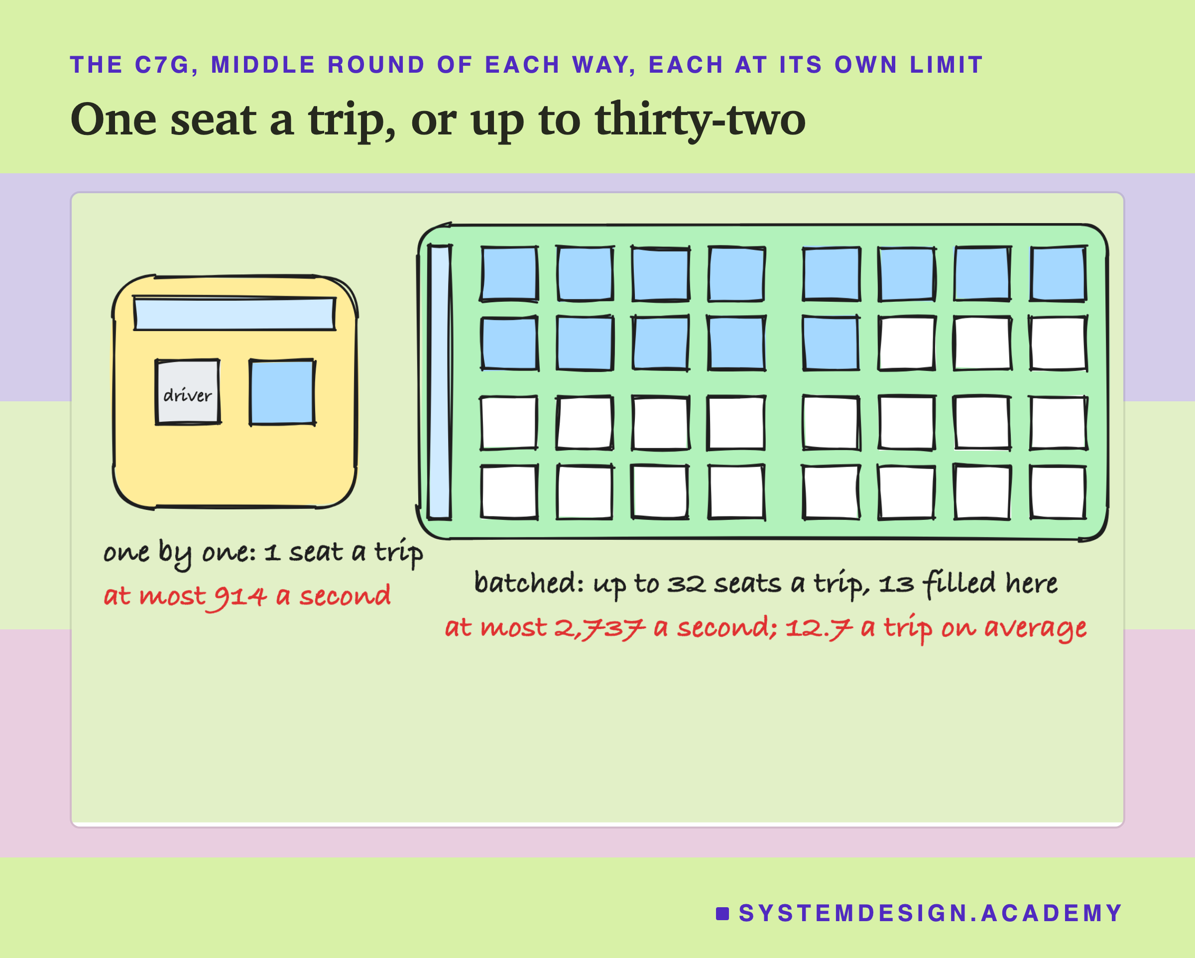
Think of a taxi and a bus. One by one is a taxi with one seat: each trip carries one rider. Batched is a bus with 32 seats that leaves the moment the driver is free, with whoever is waiting. On the c7g.medium at its batched limit, a trip carried 12.7 requests on average in the middle round. The bus was well under half full and still did three times the work.
The c8g.medium and c7a.medium were too close to call in rate, both one by one and batched: their sets of 5 overlapped each time.
Five Piles of Coins
The shelf labels gave the headline. This slide shows how the five boxes compare with each other.
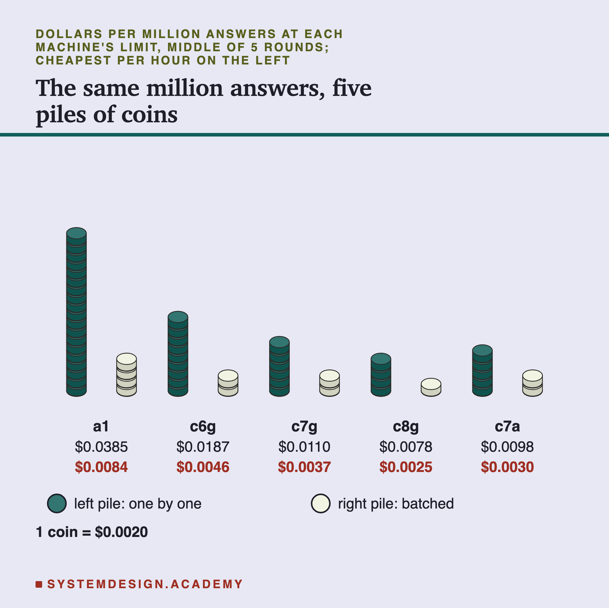
Read left to right, the sticker price per hour goes up, but the piles do not shrink in step. The a1.medium's left pile towers over the rest.
The c7a.medium costs the most per hour, $0.0513. One by one it reached 1,453 a second against the c8g.medium's 1,428, too close to call. Its price is 29% higher, though, so per answer it came out dearer, and that difference was clear in every round.
For every pair of boxes, both arms, the two sets of 5 costs did not overlap, so all 20 comparisons are clearly different. Even so, batching moved costs more than the choice of box did. The dearest box batched, the a1.medium at $0.0084, cost only a little more per answer than the cheapest box one by one, the c8g.medium at $0.0078.
These costs share the tester's handicap from the headline: 4 to 9% of the core went to the tester one by one, 13 to 19% batched.
Who Used the One Core
The tester and the service shared one core, as in every lesson of this chapter. So how much of the core did each get?
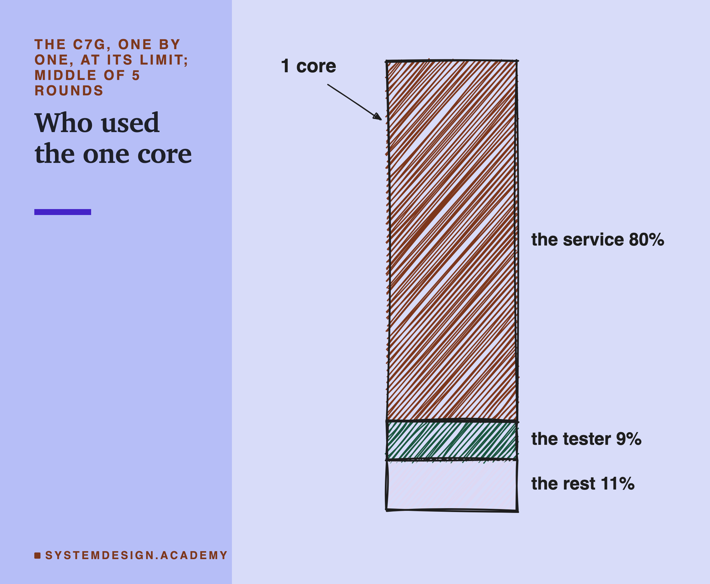
This is the c7g.medium, one by one, at its limit, in the middle round. Processor time is the time the chip spent running a program. I read the tester's and the service's processor time during the counted 12 seconds and divided each by the 12 seconds. The service used 80% of the core and the tester 9%. The rest, 11%, went to the system, other programs, or nothing at all. The three parts add up to the whole core.
I had guessed the tester would take at least a quarter. That guess was wrong: one by one it took 4 to 9% on the five boxes. Batched it took more, 13% on the a1.medium up to 19% on the c7g.medium, because it sent three to four and a half times as many requests.
The limit came before the core was full. Over each whole run, Linux counted the core as idle about 10% of the time on the c7g.medium at its one-by-one limit, and about 30% on the a1.medium. So the slowest 1 in 100 went over 25 ms with time to spare. Requests arrive at random and sometimes bunch up, and on one core a bunch must wait in line, as lesson 3 showed.
In a real setup the users would be on their own computers, and the service would get the tester's share too. I did not measure how much faster it would then be, so I add nothing. My costs are pessimistic, more so for batching.
Why Real Services Run Below Their Limit
So far every cost assumed a box busy at its limit every second. No real service runs like that. I can show two reasons with this lab's own data, and add a third that is common sense rather than measurement.
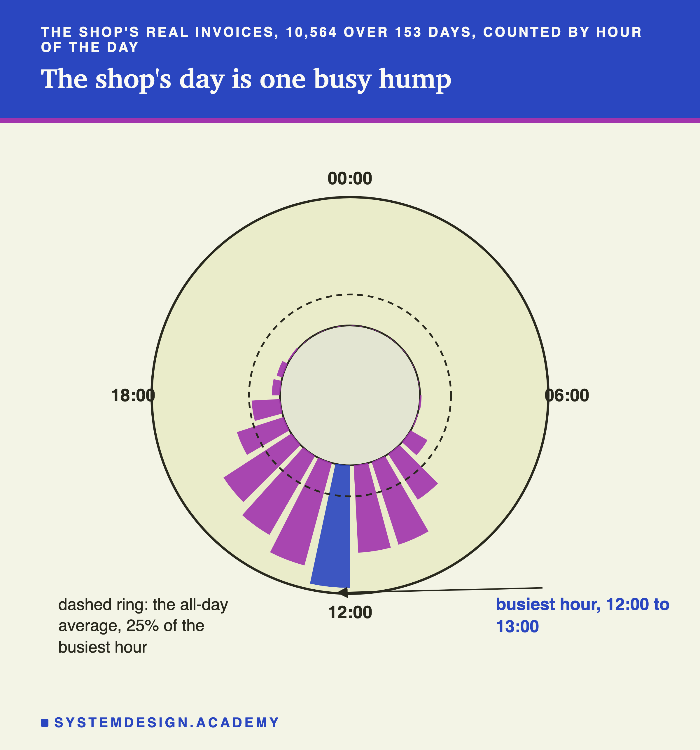
The first reason is that traffic has a shape. An invoice is the bill for one order, and this clock counts the shop's real invoices from July to November 2011 by hour of the day. Almost nothing happens at night. The busiest hour, 12:00 to 13:00, had 11.4 invoices on an average day. Over all 24 hours the average was 2.9 an hour, 25% of the busy hour.
A service must be big enough for its busiest hour. Say you size a box for this shop's average busiest hour. Then over the whole day it does on average only a quarter of the work it could do. Real busy days, and busy minutes inside the busy hour, run higher than that average, so the true share is lower still. And the shop's actual numbers are tiny, 11 invoices an hour is far below any box's limit; what carries over is the shape of the day.
The second reason comes from the staircase. On the c7g.medium's batched search, the scout's quick first climb, not a counted run, saw the slowest 1 in 100 at 2.3 ms at 400 requests a second. On the limit's own step, in counted runs, it was 13 to 16 ms. A service run near its limit is one burst away from the cliff.
The third is common sense: boxes break and traffic grows. With two boxes, if one fails the other must carry everything, which only works if each normally runs below half its limit.
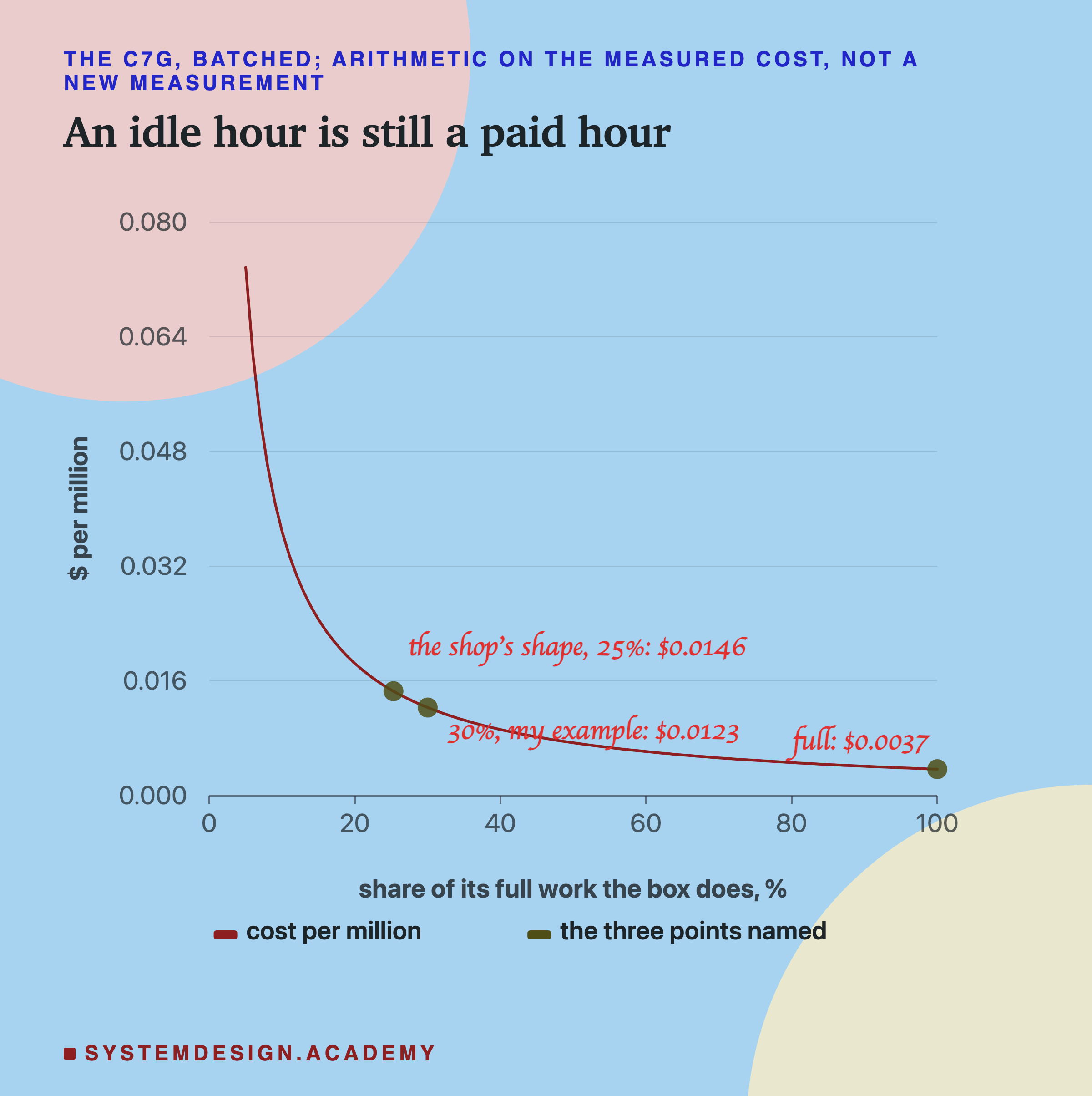
The price per hour does not change when the box is idle. So the cost per answer is the cost at the limit divided by the share of work the box does. Half the work means twice the cost per answer. This curve is arithmetic on the measured cost, not a new measurement.
Always On, or Once a Night
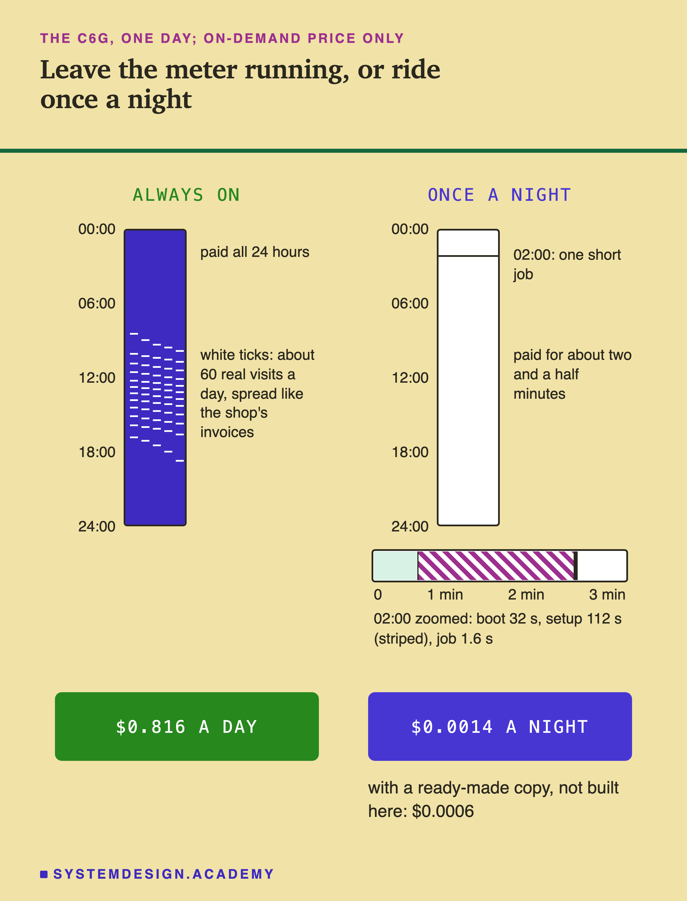
Lesson 1 offered the other way: score everyone once a night and keep the scores. What does that cost? I priced it on the first box, the c6g.medium, because its setup was recorded and timed.
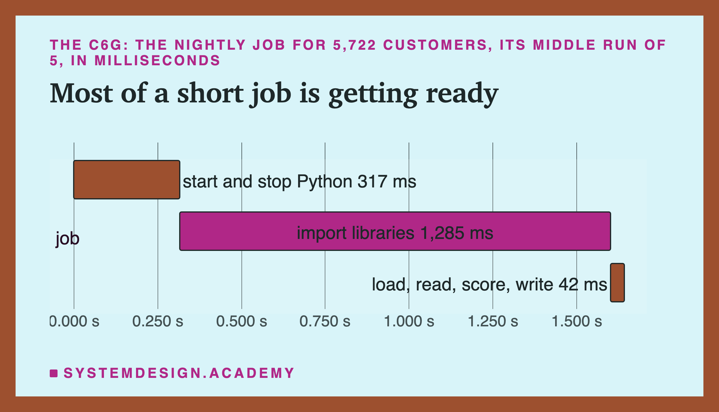
A fresh Python program started and imported its libraries, which means loading their code into memory before it can be used. It loaded the model, read all 5,722 customers' numbers for 1 November 2011 from the small database, scored them all in one call, and wrote the scores. In its middle run the whole program took 1.64 seconds, timed from outside. Importing took 1,285 ms of that, as lesson 6 found, and the scoring itself 22 ms. Every one of the job's scores was equal to the box's reference scores, to the last bit, in every round on every box.
Now the bill. AWS's on-demand page says you pay "by the hour or second (minimum of 60 seconds)". A box rented only for this job must also start, and the c6g.medium took 32 seconds from launch until SSH answered. My boxes started from plain Ubuntu, so before the job they also needed Python, the packages and the files: step 5, which took 111.5 seconds. That step also made this lab's reference scores, which a nightly job would not need. So a real job's setup would be a little shorter, but I did not time it separately. Boot, setup and job together come to about 145 seconds: $0.00137 a night.
A ready-made copy of the box could already hold Python, the model and the data. Then boot plus the job would be under a minute, and the bill would be the 60-second minimum, $0.00057 a night. I did not build such a copy, so that number is worked out, not measured, and it leaves out the small monthly charge for storing the copy.
The Same Answers on Every Chip
A cheaper box is only cheaper if it gives the same answers, so I checked.
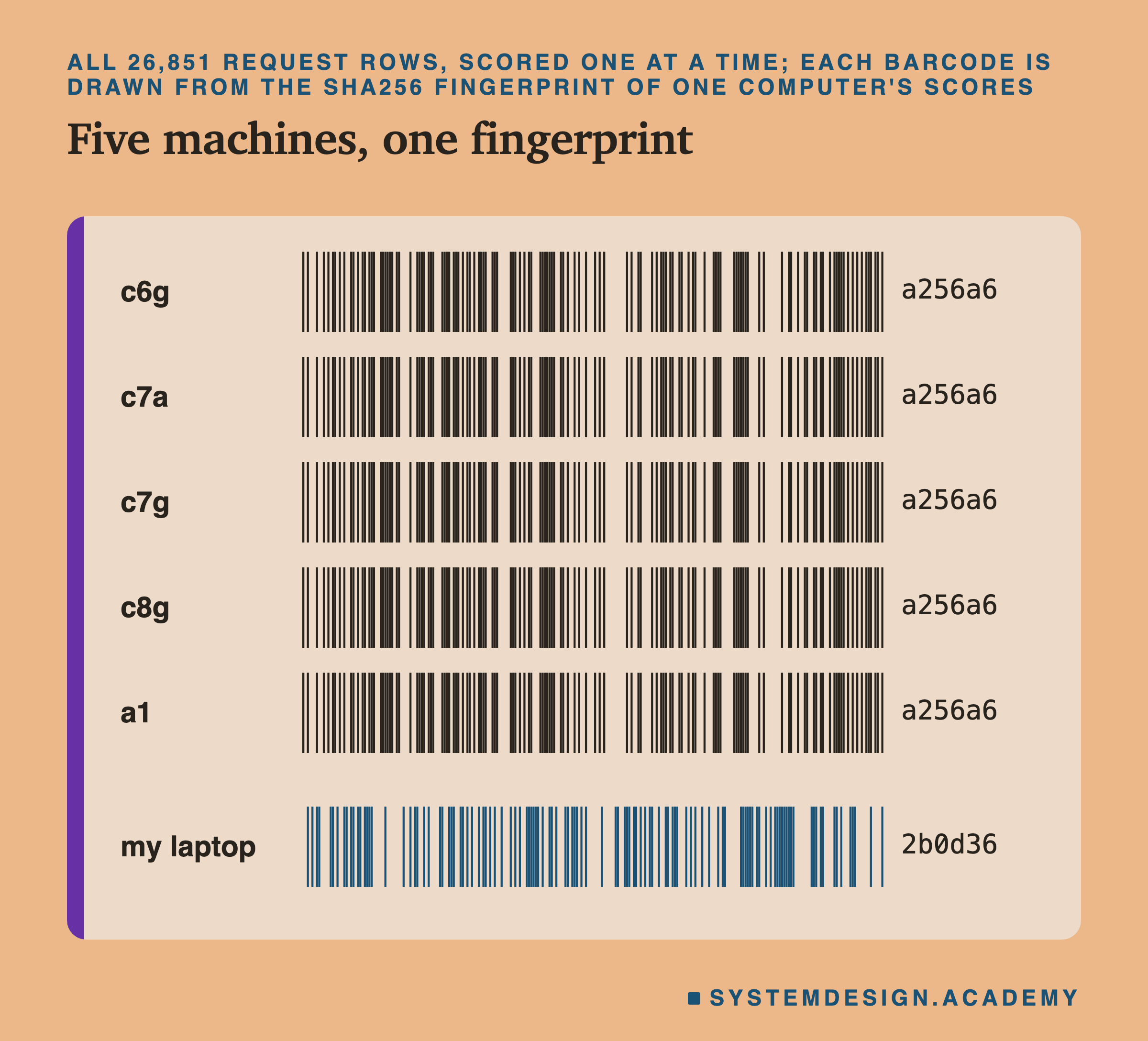
On each box, I scored all 26,851 request rows one at a time, the service's way, and again all at once in one call. Then I compared each box's one-at-a-time scores with the c7g.medium's.
All five boxes gave identical scores, to the last bit. They matched the c7g.medium on every row, so their fingerprints match. On every box, the all-at-once scores matched the one-at-a-time scores. And every answer the service gave in every run matched its box's reference: 12,700,169 answers, none different.
I had guessed that the AMD box would differ from the Arm boxes in the last digits, because the two kinds of chip can round some sums differently. That part of my guess was wrong. The one difference I found was elsewhere: all five boxes differed from lesson 2's laptop scores on 33 rows, as step 5 showed.
Bigger Boxes, Priced but Not Measured
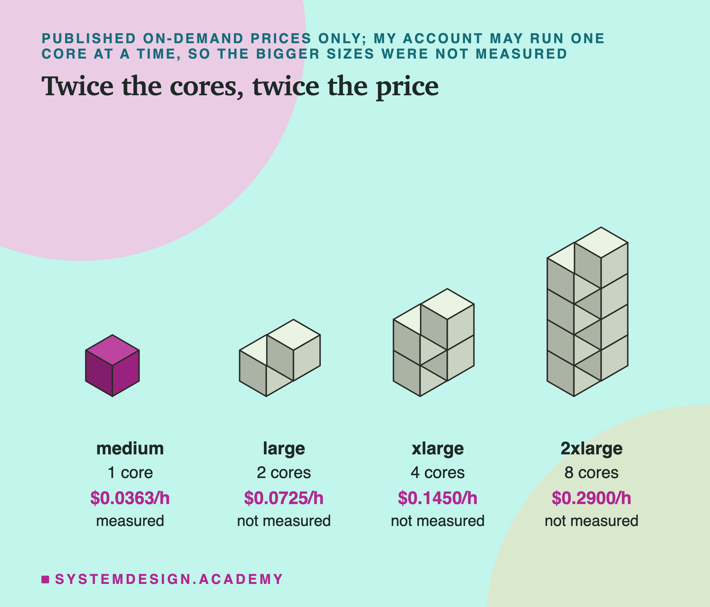
My account can run only one core at a time, so I could not test bigger boxes. AWS sells each family in sizes, and each size up has twice the cores. Here are the next three after the one I used, with their published on-demand prices. None of the bigger ones was measured.
The price doubles with the cores: $0.0725 for 2 cores, $0.1450 for 4 and $0.2900 for 8. So one core has almost exactly one price at every size. A bigger box is only cheaper per answer if your service keeps all its cores busy, for example with one copy of the service for each core. Lesson 5 could not test that on one core, and I do not guess a number.
A Month's Bill, Line by Line
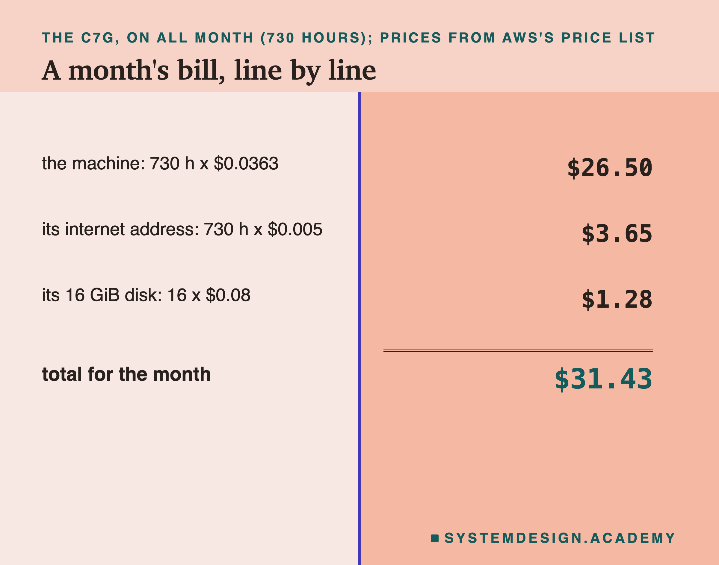
What would one always-on c7g.medium cost for a month? A month is about 730 hours, so the box itself is 730 hours times $0.0363. AWS also charges for its public internet address, $0.005 an hour, and for its 16 GiB disk, $0.08 per GB per month. All three prices come from AWS's price list.
The three lines add up to $31.43 a month, and the box itself is 84% of that. My costs per million so far used the box's price alone. With the address and the disk added, the c7g.medium's cost per million one by one rises from $0.0110 to $0.0131. The results file holds the full figure for every box. None of this counts traffic sent out of AWS, which this lab did not use.
My Twelve Guesses Before the Run, Checked
I wrote twelve guesses into the lab before it ran. Each is quoted word for word from the docstring, with a short note on its words. Seven were right, three were partly right and two were wrong. In the guesses, "none" means one by one, "batch" means batched, and a "box" is a rented computer.
-
"G1. c7g.medium, none: max rate between 850 and 1,050 a second in every round (lesson 4: 879 passed, 1,098 failed)." Right: 861, 861, 914, 914 and 914.
-
"G2. On every box, batch's max rate is at least 2 times none's, in every round." Right: 2.77 to 4.88 times, round by round.
-
"G3. c7g.medium, batch: max rate between 2,500 and 4,000 a second in every round." Right: 2,737, 2,577, 2,737, 2,737 and 2,577.
-
"G4. none's max rate orders the boxes c7a > c8g > c7g > c6g > a1, each neighbour pair clearly different." A neighbour pair is two boxes next to each other in that order. Partly right. The order held in the middle rounds: c7a 1,453, c8g 1,428, c7g 914, c6g 506, a1 184. But the c7a.medium and c8g.medium were too close to call; the other three pairs were clearly different.
-
"G5. The cheapest box per hour (a1.medium) is NOT the cheapest per 1,000 predictions, for either arm; a1.medium costs more per 1,000 than c7g.medium, clearly different, for both arms." Right. It was the dearest of all five per answer.
-
"G6. c7g.medium, none, at the limit: between $0.0000080 and $0.0000140 per 1,000 predictions (median of rounds)." The median is the middle value. Right: $0.0000110.
-
"G7. Every served score equals its box's single-row reference to the bit, and all.npy equals ref.npy on every box. The four Arm boxes' ref.npy are identical to the bit; c7a.medium (x86) differs from c7g.medium in at least one row, by at most 1e-15." Here all.npy and ref.npy are the scores made all at once and one at a time, and 1e-15 is a millionth of a billionth. Partly right. Every served score matched, all at once matched one at a time on every box, and the four Arm boxes matched each other. The wrong part: the AMD box did not differ at all.
How I Would Price a Model Service
If I had to price a prediction service tomorrow, this is the order I would work in, with this lab's numbers as the example.
-
Write down the target. Mine was: the slowest 1 in 100 within 25 ms. A different target gives a different rate, and so a different cost.
-
Measure the rate on the box you will rent, with an honest tester. Send requests at planned random times, time each answer from its planned arrival, climb in small steps, and repeat the climb. The knee is sharp: on the c7g.medium batched, one step past the limit took the slowest 1 in 100 from 13 to 16 ms to at least 63 ms.
-
Divide. Price per hour, divided by answers per hour, times 1,000. Then read the unit price, not the sticker.
-
Turn on batching before you buy a bigger box. Here it gave 3.0 to 4.6 times the answers for no extra money.
-
Divide again by how much of its work the box will really do. You must size for the busy hour. For a day shaped like this shop's, the box does about a quarter of its work, so the cost per answer is about four times the cost at the limit.
-
Price the nightly job too. If a score a day old is good enough, one short job a night costs about $0.0014 on the c6g.medium as I built it, and less with a ready-made copy.
Try It Yourself
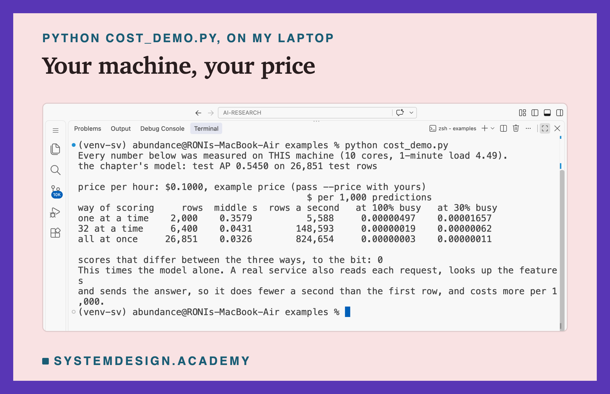
The full lab needs five rented boxes for about three and a half hours in all. The demo, cost_demo.py, runs on your own computer. It times the model alone in three ways and turns your own speed into a cost per 1,000, at a price you type in.
I wrote the demo's design into its docstring after the lab's design and before the demo first ran.
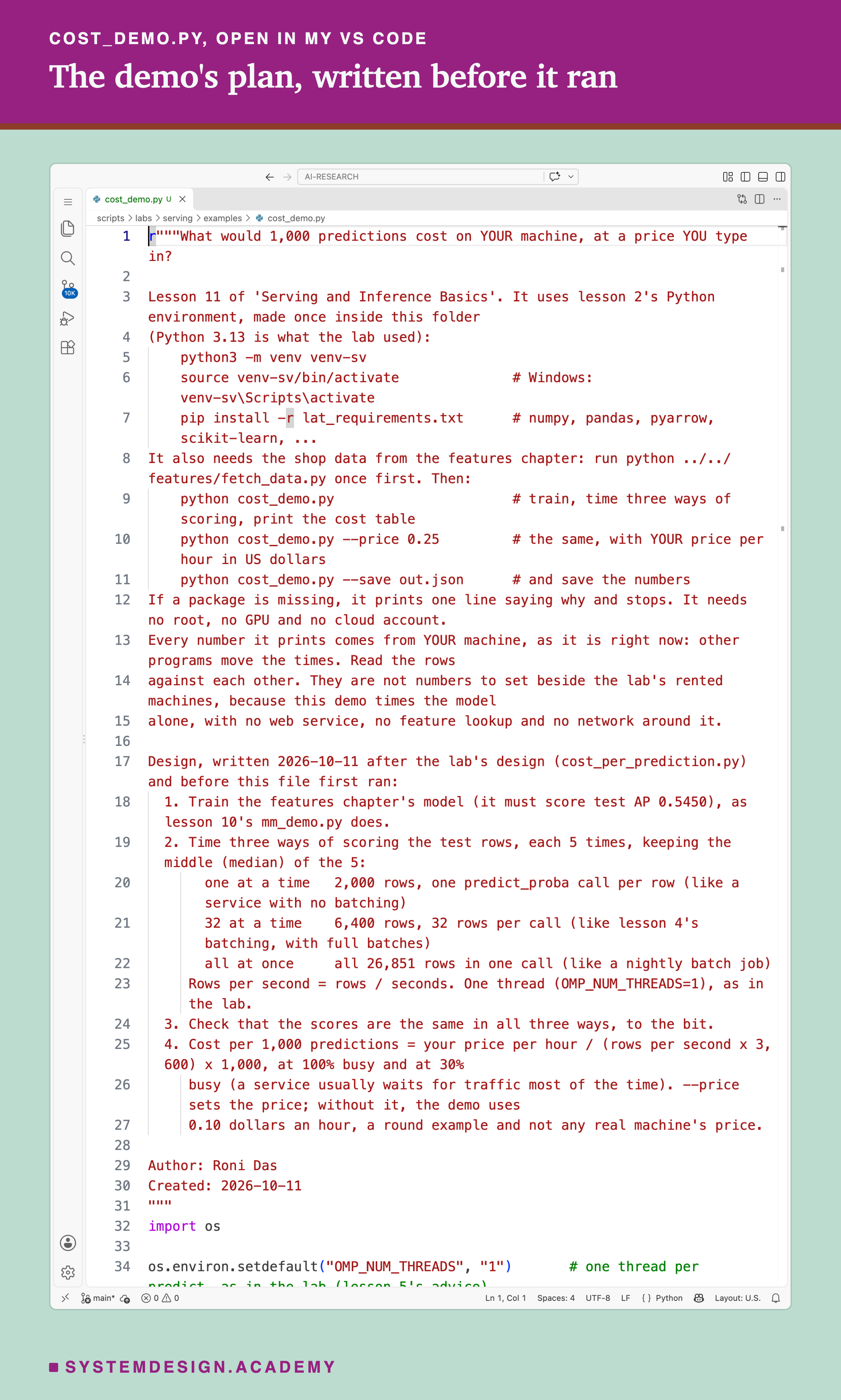
Before you run this lab. The demo uses lesson 2's venv, with the library versions of the lab's boxes. If you made it for lessons 2 to 10, use it again. If not, make it once, inside the scripts/labs/serving/examples folder:
python3 -m venv venv-sv
source venv-sv/bin/activate        # on Windows: venv-sv\Scripts\activate
pip install -r lat_requirements.txt
I used Python 3.13. Then run python ../../features/fetch_data.py once, which downloads the shop data. Now run python cost_demo.py. To use your own price, add --price and the dollars per hour, such as python cost_demo.py --price 0.25. It needs no graphics card, no cloud account and no administrator rights. If a package is missing, it prints one line saying why and stops.
Its first line says the numbers come from your computer, with its number of cores and its load at that moment. The demo times the model alone, with no web service around it, so its numbers are not the lab's numbers. Read its three rows against each other.
r"""What would 1,000 predictions cost on YOUR machine, at a price YOU type in?

Lesson 11 of 'Serving and Inference Basics'. It uses lesson 2's Python environment, made once inside this folder
(Python 3.13 is what the lab used):
    python3 -m venv venv-sv
    source venv-sv/bin/activate              # Windows: venv-sv\Scripts\activate
    pip install -r lat_requirements.txt      # numpy, pandas, pyarrow, scikit-learn, ...
It also needs the shop data from the features chapter: run python ../../features/fetch_data.py once first. Then:
    python cost_demo.py                      # train, time three ways of scoring, print the cost table
    python cost_demo.py --price 0.25         # the same, with YOUR price per hour in US dollars
    python cost_demo.py --save out.json      # and save the numbers
If a package is missing, it prints one line saying why and stops. It needs no root, no GPU and no cloud account.
Every number it prints comes from YOUR machine, as it is right now: other programs move the times. Read the rows
against each other. They are not numbers to set beside the lab's rented machines, because this demo times the model
alone, with no web service, no feature lookup and no network around it.

Design, written 2026-10-11 after the lab's design (cost_per_prediction.py) and before this file first ran:
  1. Train the features chapter's model (it must score test AP 0.5450), as lesson 10's mm_demo.py does.
  2. Time three ways of scoring the test rows, each 5 times, keeping the middle (median) of the 5:
       one at a time   2,000 rows, one predict_proba call per row (like a service with no batching)
       32 at a time    6,400 rows, 32 rows per call (like lesson 4's batching, with full batches)
       all at once     all 26,851 rows in one call (like a nightly batch job)
     Rows per second = rows / seconds. One thread (OMP_NUM_THREADS=1), as in the lab.
  3. Check that the scores are the same in all three ways, to the bit.
  4. Cost per 1,000 predictions = your price per hour / (rows per second x 3,600) x 1,000, at 100% busy and at 30%
     busy (a service usually waits for traffic most of the time). --price sets the price; without it, the demo uses
     0.10 dollars an hour, a round example and not any real machine's price.

Author: Roni Das
Created: 2026-10-11
"""
import os

os.environ.setdefault("OMP_NUM_THREADS", "1")       # one thread per predict, as in the lab (lesson 5's advice)

import importlib.util  # noqa: E402
import json  # noqa: E402
import sys  # noqa: E402
from pathlib import Path  # noqa: E402
from time import perf_counter_ns  # noqa: E402

NEEDED = ("numpy", "pandas", "pyarrow", "sklearn")
missing = [m for m in NEEDED if importlib.util.find_spec(m) is None]
if missing:
    sys.exit(f"cost_demo.py needs {', '.join(missing)}: make the environment in its docstring "
             f"(pip install -r lat_requirements.txt), then run it with that environment's python.")

import numpy as np  # noqa: E402

REPEATS = 5
BUSY = 0.30


def build():
    """The features chapter's data and model (lesson 10's mm_demo.py build step)."""
    from sklearn.metrics import average_precision_score
    here = Path(__file__).resolve().parent
    sys.path.insert(0, str(here.parents[1] / "features"))
    import task
    from what_a_feature_is import HAND_COLS, hgb, joined

    ev = task.load_events()
    lab_tr, _, lab_te = task.splits(ev)
    tr = joined(ev, lab_tr, task.TRAIN_CUTOFFS)
    te = joined(ev, lab_te, task.TEST_CUTOFFS)
    X, y = tr[HAND_COLS].to_numpy(float), tr["label"].to_numpy()
    Xt = np.ascontiguousarray(te[HAND_COLS].to_numpy(np.float64))
    yt, ct = te["label"].to_numpy(), te["cutoff"].to_numpy()
    model = hgb(0).fit(X, y)
    p = model.predict_proba(Xt)[:, 1]
    ap = float(np.mean([average_precision_score(yt[ct == c], p[ct == c]) for c in np.unique(ct)]))
    assert round(ap, 4) == 0.5450, ap
    return model, Xt, ap


def timed(fn) -> tuple[float, np.ndarray]:
    """Median seconds of REPEATS runs of fn(), and the scores of the last run."""
    secs, out = [], None
    for _ in range(REPEATS):
        t0 = perf_counter_ns()
        out = fn()
        secs.append((perf_counter_ns() - t0) / 1e9)
    return float(np.median(secs)), out


def main() -> None:
    price = float(sys.argv[sys.argv.index("--price") + 1]) if "--price" in sys.argv else 0.10
    try:
        load = f"{os.getloadavg()[0]:.2f}"
    except (AttributeError, OSError):
        load = "not available on this system"
    n = os.cpu_count()
    print(f"Every number below was measured on THIS machine ({n} {'core' if n == 1 else 'cores'}, 1-minute load {load}).")
    model, Xt, ap = build()
    print(f"the chapter's model: test AP {ap:.4f} on {len(Xt):,} test rows")
    one = Xt[:2000]
    many = Xt[:6400]

    def one_at_a_time():
        return np.array([model.predict_proba(one[i:i + 1])[0, 1] for i in range(len(one))])

    def by_32():
        return np.concatenate([model.predict_proba(many[i:i + 32])[:, 1] for i in range(0, len(many), 32)])

    def all_at_once():
        return model.predict_proba(Xt)[:, 1]

    rows = {}
    s1, p1 = timed(one_at_a_time)
    s32, p32 = timed(by_32)
    sall, pall = timed(all_at_once)
    rows["one at a time"] = (len(one), s1)
    rows["32 at a time"] = (len(many), s32)
    rows["all at once"] = (len(Xt), sall)
    neq = int((p1 != pall[:len(one)]).sum() + (p32 != pall[:len(many)]).sum())

    unit = "your price" if "--price" in sys.argv else "example price (pass --price with yours)"
    print(f"\nprice per hour: ${price:.4f}, {unit}")
    print("                                          $ per 1,000 predictions")
    print("way of scoring     rows  middle s  rows a second   at 100% busy   at 30% busy")
    out = {"cores": os.cpu_count(), "load": load, "test_ap": ap, "price_per_hour": price, "repeats": REPEATS,
           "busy": BUSY, "ways": {}}
    for name, (n, s) in rows.items():
        rate = n / s
        c100 = price / (rate * 3600) * 1000
        c30 = c100 / BUSY
        print(f"{name:<14}{n:>8,}{s:>10.4f}{rate:>15,.0f}{c100:>15.8f}{c30:>14.8f}")
        out["ways"][name] = {"rows": n, "median_s": s, "rows_per_s": rate, "usd_per_1000": c100,
                             "usd_per_1000_at_30pct": c30}
    print(f"\nscores that differ between the three ways, to the bit: {neq}")
    print("This times the model alone. A real service also reads each request, looks up the features")
    print("and sends the answer, so it does fewer a second than the first row, and costs more per 1,000.")
    out["scores_neq"] = neq
    if "--save" in sys.argv:
        Path(sys.argv[sys.argv.index("--save") + 1]).write_text(json.dumps(out, indent=1))


if __name__ == "__main__":
    main()
Price a Day of Traffic
This box runs in your browser and needs nothing but Python. It is a calculator with a make-believe day of traffic. It uses the real rates each box reached in the lab and AWS's real prices. The day's shape follows the shop's invoices by hour. Everything else is made up: the size of the busy hour, 20,000 requests a second, and the random ups and downs.
Press Run. Then set FOLLOW_TRAFFIC = True, which changes the number of boxes every hour instead of keeping enough for the busy hour all day, and watch the bill. Try BOX = "a1.medium" and ARM = "none". One seed is luck, so try SEED = 1 to 5. The seed fixes the dice: each hour has its own dice, so changing BOX or ARM does not change the traffic.
The report script writes the boxes' real rates and prices, and the shop's invoices by hour, into this box from the lab's results. As shipped, the c7g.medium batched needs 9 boxes for the busy hour. Kept all day, they do 20 to 21% of their work over seeds 1 to 5. Following the traffic, the boxes do 66 to 67%, and with seed 1 the day's bill falls from $7.84 to $2.47.
The calculator is simpler than real life in three ways. It adds a tenth to every hour's need for bad luck, which is my choice and not a rule. It changes the number of boxes instantly, while a real box took about half a minute to start in this lab. And it assumes a box at its limit keeps its slowest 1 in 100 under 25 ms, which the lab measured only in 12-second runs.
The Lab's Code, Piece by Piece
The lab has files that run on my laptop, small files that run on the rented boxes, and the step script you saw above.
cost_per_prediction.py, on my laptop, holds the design and my guesses in its docstring, written before any run. Its commands: check makes sure every file is present; prices reads AWS's price list; status reads a box's console; cost works out one box's bill and checks that everything was deleted; collect gathers every box's raw files into the results; and factcheck looks up each quoted sentence in its source. collect calls cost_stats.py, which copies the raw files into results/cost-raw/, passes every log line through cost_redact.py to black out private details, keeps a small summary of each run, and does the arithmetic.
On the boxes, cost_files/cost_client.py is lesson 7's tester, with lesson 7's pauses taken out. cost_files/cost_ref.py makes the reference scores. cost_files/cost_batch.py is the nightly job in a fresh program. cost_files/cost_run.sh wraps every run: it waits for an idle core, starts a fresh service, and records the load and the system's log. does the scout, fixes the ten rates, and runs the 5 rounds, each in its own shuffled order. The service itself is lesson 4's , copied unchanged, which loads lesson 2's .
When to Use Each One, and When Not To
An always-on service is right when answers must be fresh, such as a score that depends on what the customer did a minute ago. It also needs traffic steady enough to keep the box busy. With thin traffic it is wrong: for this shop, one always-on box would cost $13.56 per 1,000 answers asked for.
A nightly batch job is right when a score a day old is good enough, as lesson 1 found for this shop. You must also be able to list everyone who needs a score. It is wrong when most scores are never read and the list is huge, or when a new customer needs a score before tonight.
Batching inside the service is right on any service that gets more than a few requests at a time. Here it gave every box three to four and a half times the answers for no extra money. When two requests almost never wait together, it neither helps nor hurts much.
Choosing a box by its hourly price alone is never right. Measure the rate on the real box with the real model, then divide.
What This Lab Cannot Tell You
The model is small. It is a tree model, which scores a customer by asking a chain of yes-or-no questions about their numbers, and it ran on a CPU. A neural network is a much bigger kind of model, usually run on a graphics card, and its cost per answer can be very different. Other boxes would win.
I rented one box of each type. Another box of the same type, on other hardware in the data centre, may be a few percent faster or slower. On the c7g.medium, the one-by-one limit here agrees with lesson 4's, measured on a different box.
Only one-core boxes could run, because my account allows one core at a time. Bigger boxes are priced but not measured.
The tester shared the core, so every rate includes its share and the costs are a little high, batched ones more.
I used on-demand prices only. AWS also sells cheaper ways to rent. One is a lower price for a one- or three-year promise; another is spare boxes that AWS may take back at short notice. I did not test those and do not quote their prices.
Traffic was steady and random for 12 seconds at a time. Real traffic rises and falls; the busy-hours slide prices that only with arithmetic.
The nightly bill with a ready-made copy of the box is worked out, not measured.
During the run I changed the demo's printing twice on the first box, as step 11 explains. Nothing else changed after the first box's schedule started. After an independent review, I added the setup time to the nightly bill and the idle share to the core slide. I also added the two scripts that drove the four unrecorded boxes.
What to Do on Monday
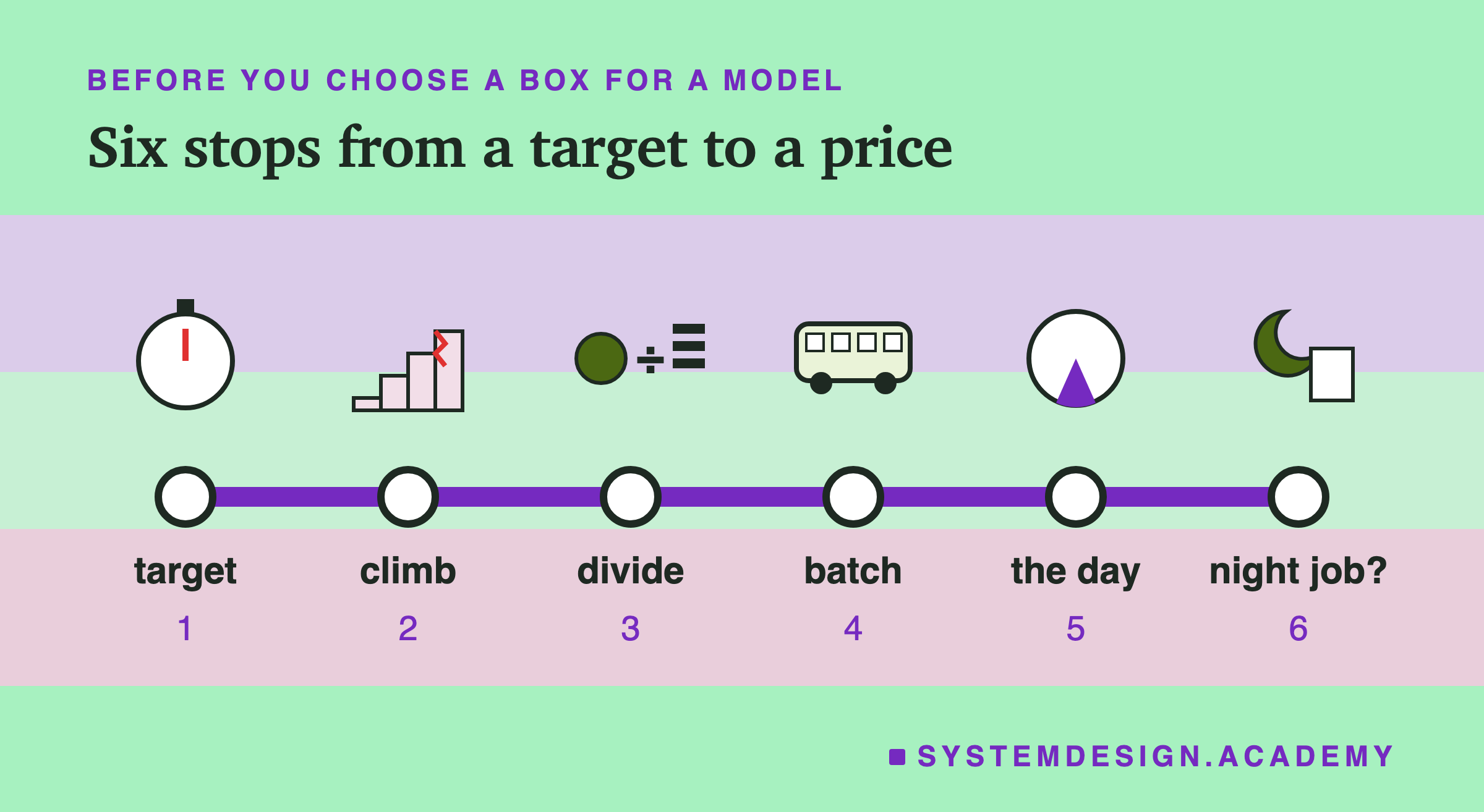
On Monday, start at stop 1: write down the slowest wait your users will accept. Then climb, on the box you rent and with your own model, until you find the highest rate that keeps it. Divide the hourly price by the answers in an hour.
Stops 4 to 6 are cheap to try. Turn on batching if your service can get more than one request at a time. Look at how much of its work your box really does across a day. And if it is idle most of the day and the answers can wait until morning, price a nightly job instead.
The price of a box is the sticker; the answers it gives in an hour are the weight. Read the unit price.
Knowledge Check
Knowledge Check
4 questions - Score 80% to pass
The a1.medium had the lowest price per hour of the five boxes. Why was it not the cheapest per million answers?
On the c7g.medium, batching let the service take about three times as many requests a second. What made that possible?
A box rented only for the nightly job did about one second of work. Why could the bill be the 60-second minimum?
A box sized for the shop's average busiest hour does, over the day, a quarter of the work it could do. What does that do to its cost per answer?