Imagine a small team that ships parcels along one regular route, through many ports and cities around the world. Every week the same kind of parcel leaves the warehouse, passes the same places, and a report comes back. At the end of a long season the team leader pins a large world map to the wall and asks everyone to stick a pin wherever something went wrong: the port that closed in a storm, the customs office that wanted a form nobody had filled in, the depot whose clock ran an hour behind, the address that no longer existed.

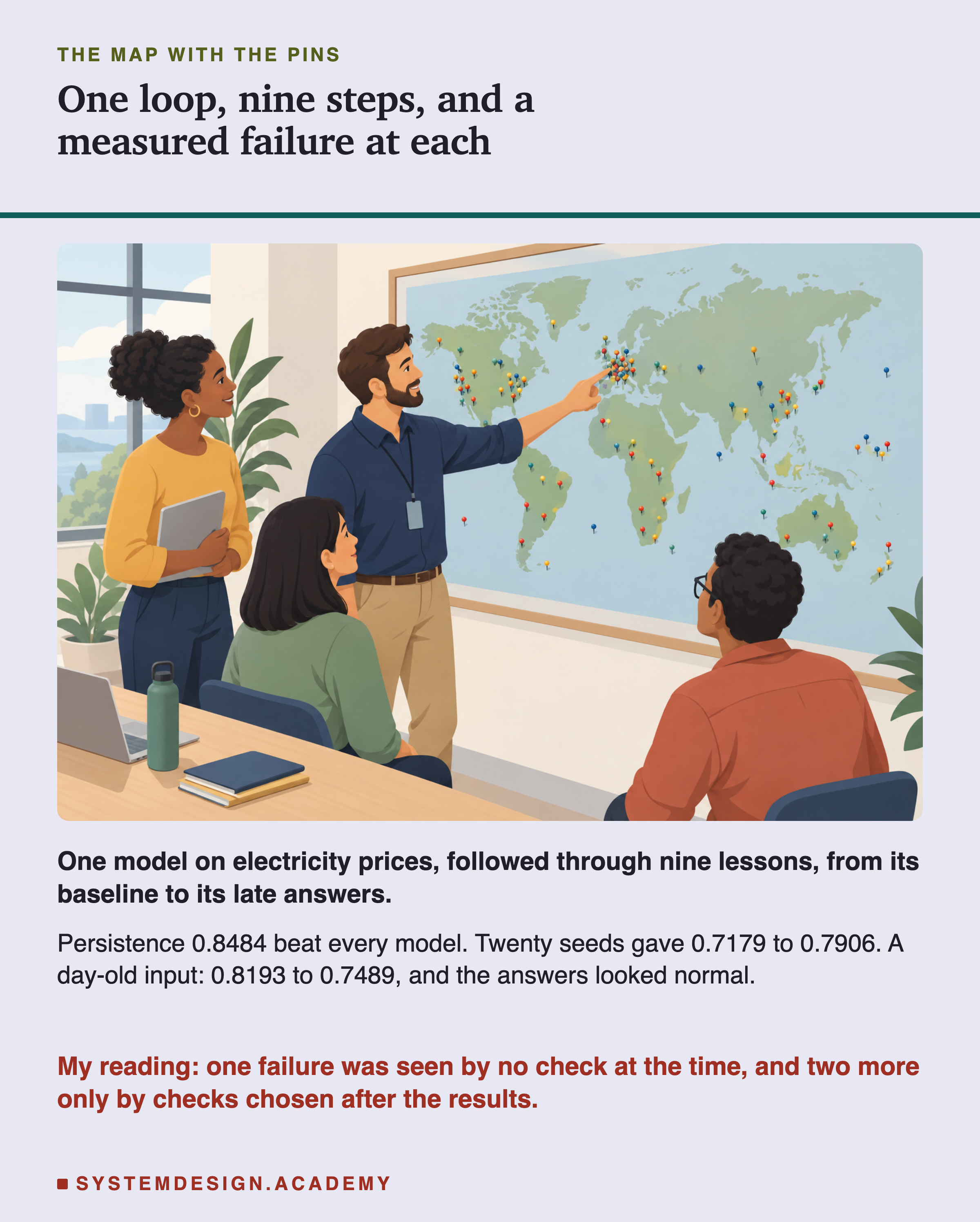
The pins are useful because each one is a real event, with a date and a story, not a guess about what might go wrong. But the leader also notices something about the map. Some pins were found by a check the team already ran, such as the morning look at the weather reports. Other pins were found by nobody at the time. The depot's slow clock, for example, was only noticed weeks later, when the complaints came in.

So the leader does two things. She walks the route once on the map, in the order a parcel travels it, and at each pin she asks: what is this stop for, what went wrong here, what would have told us sooner, and what do we still not know about it? Then she writes one page of checks that the next season's team can keep by the door.

This lesson does the same for a program that learns from examples. The chapter followed one such program through nine lessons, and each lesson put a pin in the map. Here I walk the whole route once, in order, and then write the one page.

This is the last lesson of the chapter. Over nine lessons I followed one kind of program, trained on the same public record of electricity prices, from the first question anyone should ask about it to the problems that only appear months after it is in use. Each lesson took one step of that life and measured, on the data, what goes wrong at that step.

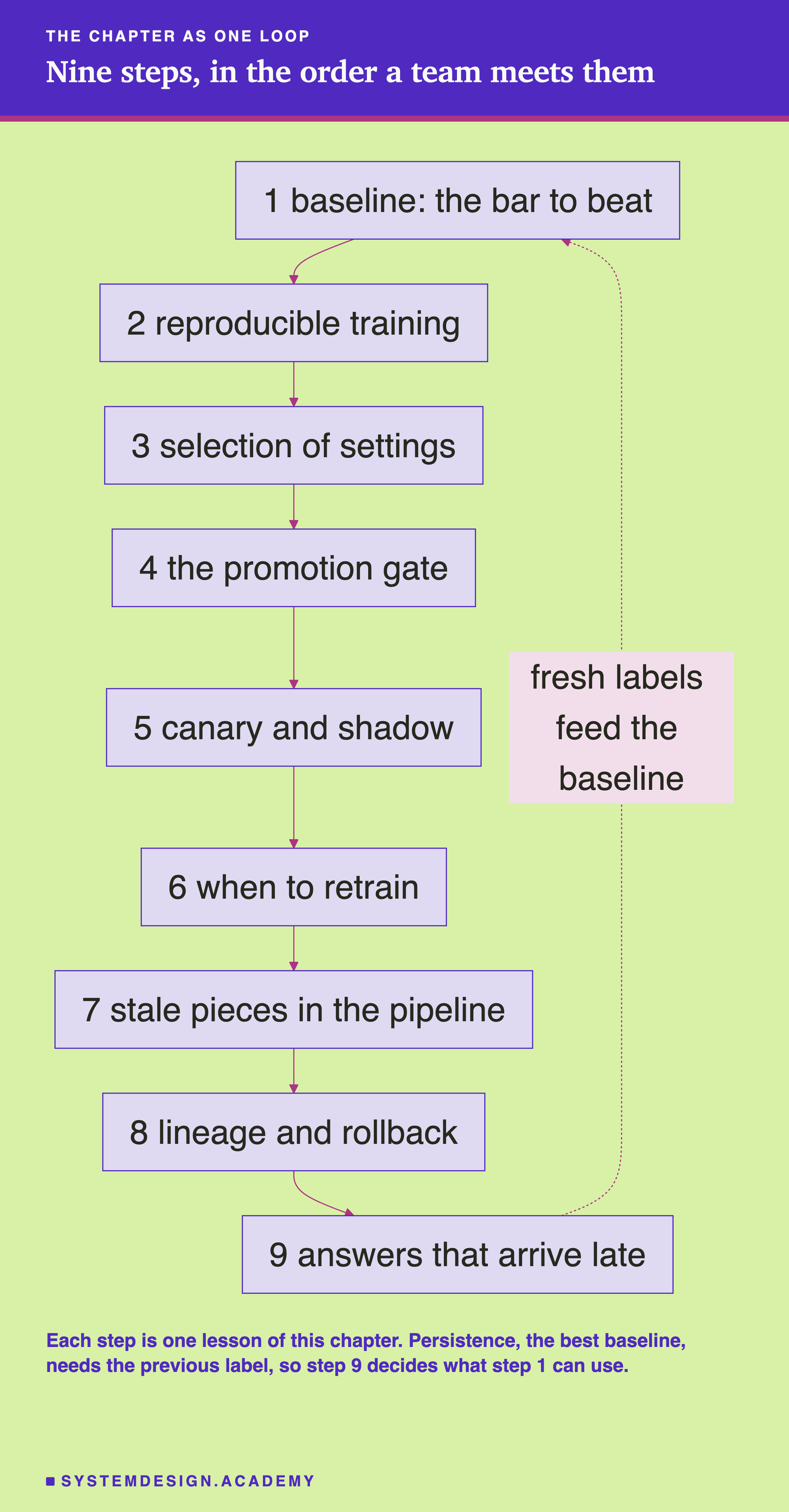
The nine steps, in the order a team meets them, are the nine lessons: start with the dumbest model, same code, different model, picking the best of many, the promotion gate, canary and shadow, when to retrain, stale pieces in a pipeline, lineage and rollback and when the answers arrive late.

They form a loop, not a line. Once a program is in use, new answers come back, it is trained again, judged again and put back into use, and the same nine questions come round again. The last step also feeds the first in a very direct way on this data, which a later slide shows.

The course's lesson on training pipelines and orchestration explains in words how software runs such a loop. The chapter before this one ended with its own checklist, a production readiness check, built on bike rentals. This lesson does not repeat either. It reads this chapter's nine results back as one route.

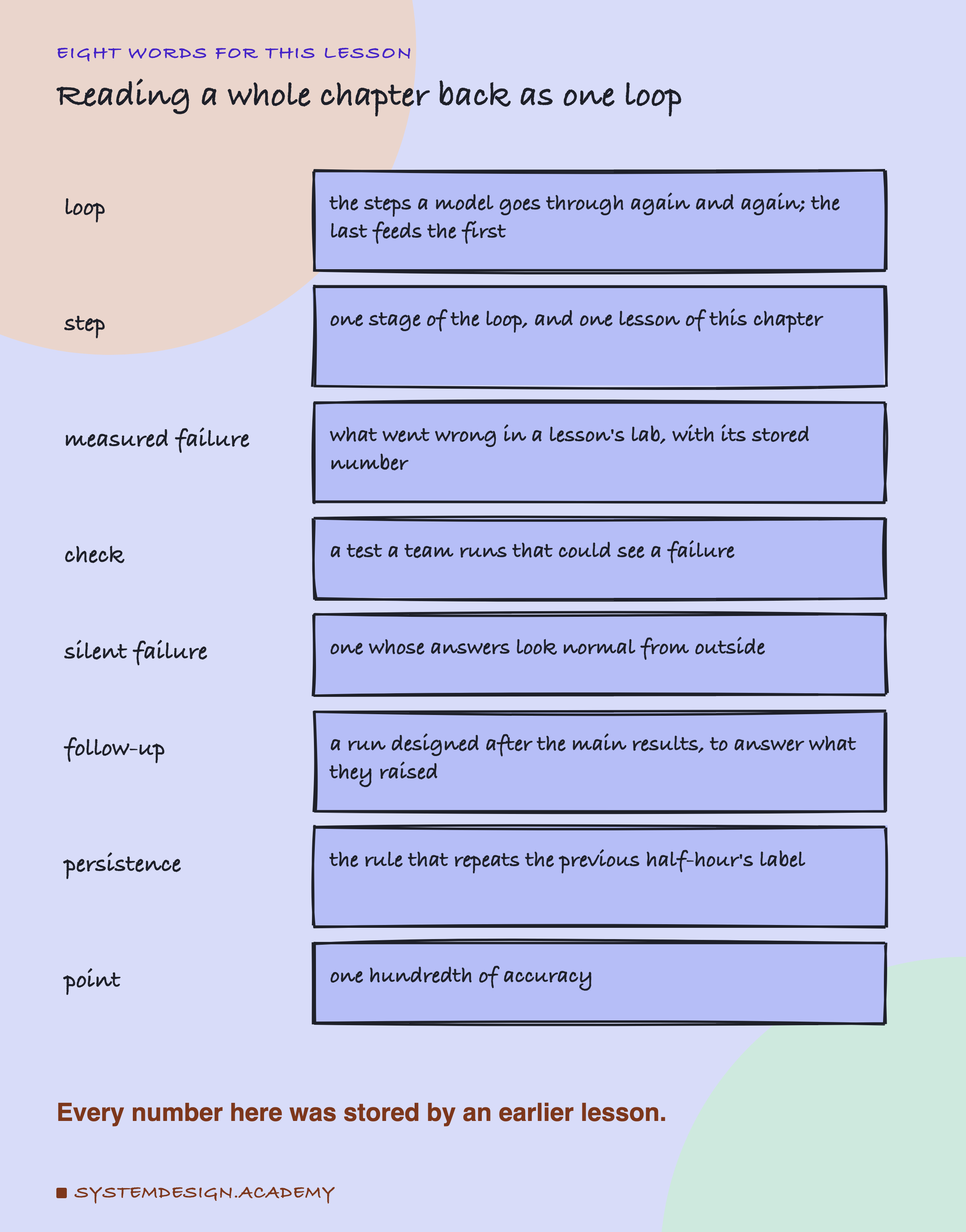
A model is a program that learned from examples. In this chapter it answers one question for each half-hour of the electricity market: is the price UP or DOWN compared with its average over the last 24 hours? That right answer is the half-hour's label. Accuracy is the share of half-hours a model got right, and a point is one hundredth of accuracy, so 0.75 to 0.78 is 3 points.

The loop is the set of steps a model goes through again and again, with the last step feeding the first. A step is one stage of the loop, and in this chapter each step is one lesson. A measured failure is what went wrong in that lesson's lab, with the number the lab stored. A check is a test a team can run that might see a failure. A failure is silent when the model's answers look normal from outside, so nothing makes anyone look. Whether some check saw a failure in time is a separate question, and a later slide states the rule I used for it.

A follow-up is a run I designed after seeing a lab's main results, to answer a question those results raised. I wrote each follow-up's design down before it ran, but it was still chosen knowing the results, and I say so wherever one appears. And persistence is the laziest rule of lesson 1: say whatever the previous half-hour's label was.

This lesson runs no new experiment. Every number in it was stored by one of the nine earlier labs, in files under scripts/labs/lifecycle/results/. I wrote one report for this lesson, wrap_report.py, that reads those files and prints them step by step.

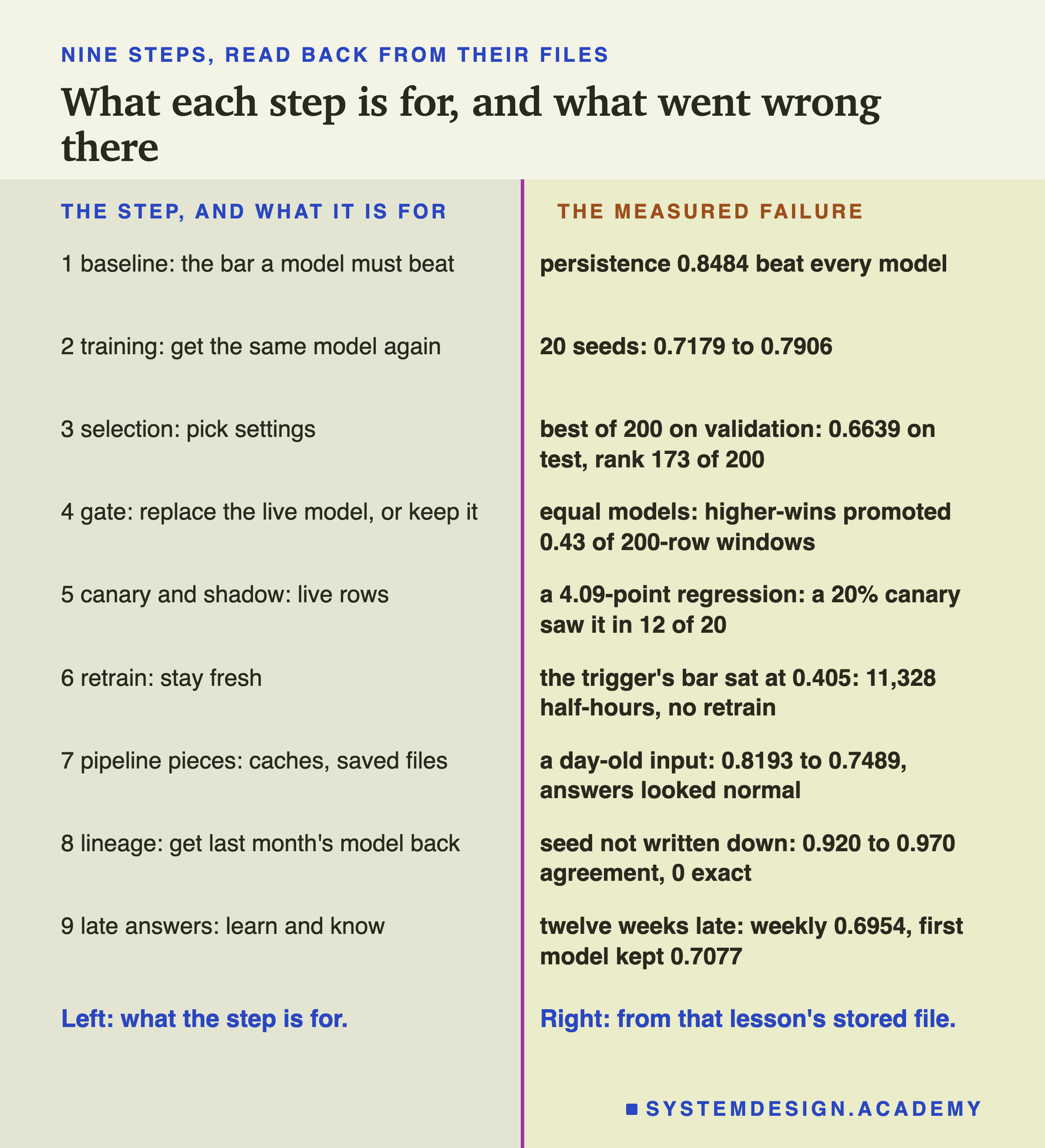
Reading numbers back is where copying mistakes creep in, so the report checks two things before it prints anything, and stops on the first mismatch. First, where a lab's own file and its lesson's report file both hold a number, the two must be equal; there are 43 such comparisons. Second, for every lesson, the report trains the lab's models again with the same data, split, settings and seeds, and at least one headline number must come back exactly, to the last digit the computer stores. There are 30 of these refit checks. For example, it trains the boosted trees with seed 0 and gets lesson 1's 0.7527 again; it plays lesson 4's coin-swap test on 20 pairs of models and gets every one of its rates again; it serves lesson 6's monthly and triggered policies again; and it retrains lesson 9's weekly model with labels twelve weeks late and gets 0.6954. All 73 checks agreed.

For each step I then answer four questions, always in the same order. What is the step for? What went wrong there, measured? What saw it, or did nothing see it? And what could the lesson not show? The first three come from the lessons. The fourth comes from each lesson's own limits slide, and I have kept the corrections those lessons made after their reviews.

What is mine, and chosen after every result was known: the order of the steps, which numbers stand for each step, the wording of each check, and a later table of which check saw which failure. Read those as my way of reading the chapter, not as a measurement.

What it is for. A trained model's score has no scale of its own. An accuracy of 0.75 is good if the laziest rule gets 0.55, and a loss if the laziest rule gets 0.85. So the first step is to score rules that learn nothing, called baselines, on the same test, and keep the best of them as the bar.

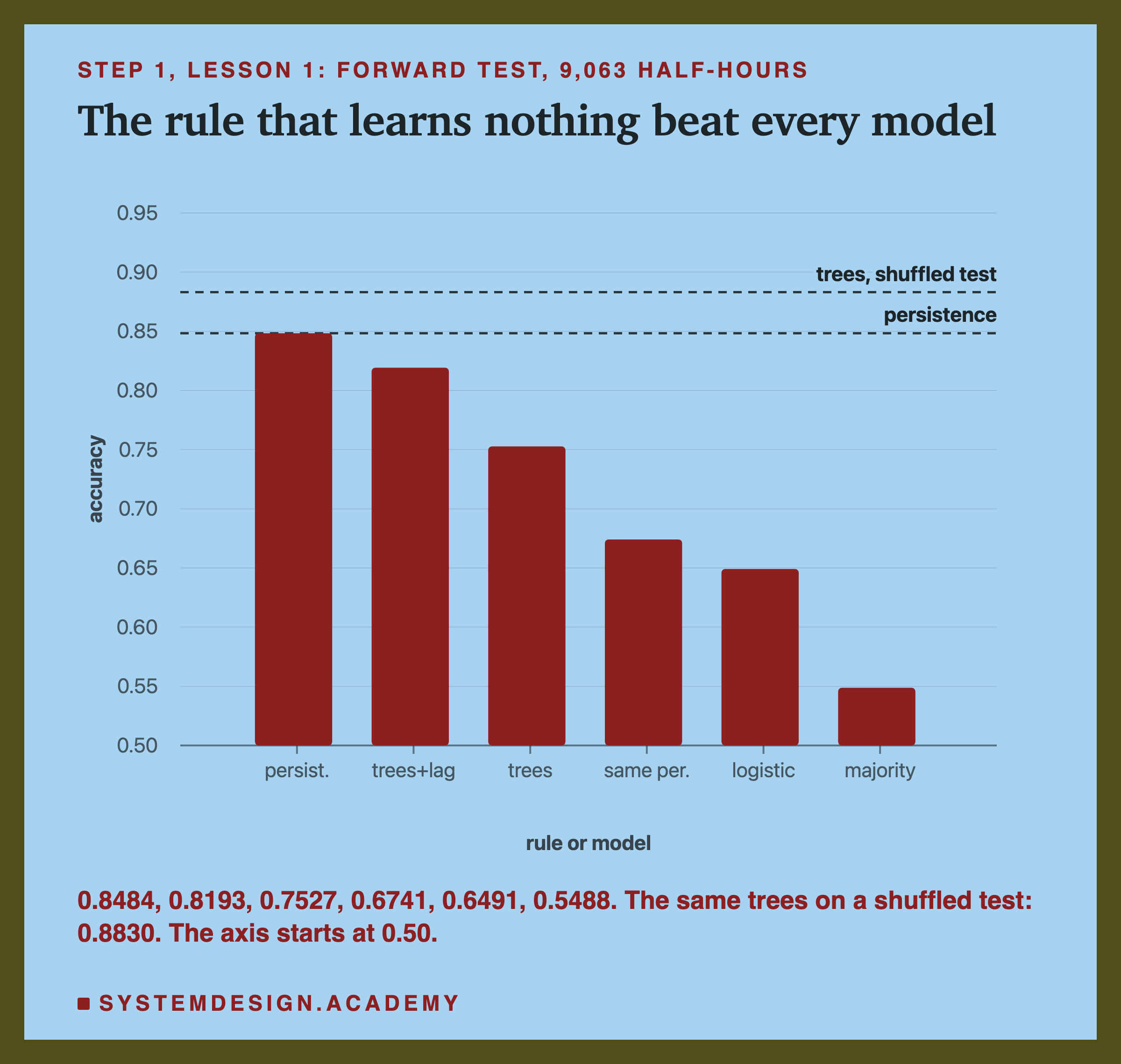
What went wrong, measured. On a forward test, the last 20% of the half-hours in time, which is the future from the model's point of view, persistence scored 0.8484. No trained model beat it. Boosted trees with the previous label as an extra input scored 0.8193, the plain trees 0.7527, logistic regression 0.6491, and the rule that always says the most common label 0.5488. The trees were not bad in general; they were worse than doing nothing clever. A follow-up, designed after the results, gave the models only the previous half-hour's market, as a strict forecast would; then the trees with the lag scored 0.8493 against 0.8484, 8 rows ahead out of 9,063, which I read as a tie. Twenty seeds of those trees, in the benchmark's framing, ran from 0.7884 to 0.8406, and none of the 20 beat persistence.

What saw it. Scoring persistence on the same forward test. Nothing else would have: the same trees tested on a shuffle of the rows scored 0.8830, and a team that tested that way would have shipped a model that loses to a one-line rule. The same lesson found where persistence fails: on exactly the 1,374 test rows where the label changed, and nowhere else.

What the lesson could not show. Whether a tuned model, or one given more lags, would beat persistence; the lab used default settings and ran each model once. And the label is sticky partly by its own definition, a price against a slow 24-hour average, so the result belongs to this data.

What it is for. A team needs to rebuild a model to debug it, to show an auditor, to roll back to it, and to compare two versions fairly. All four need a training run that gives the same model when it is run again.

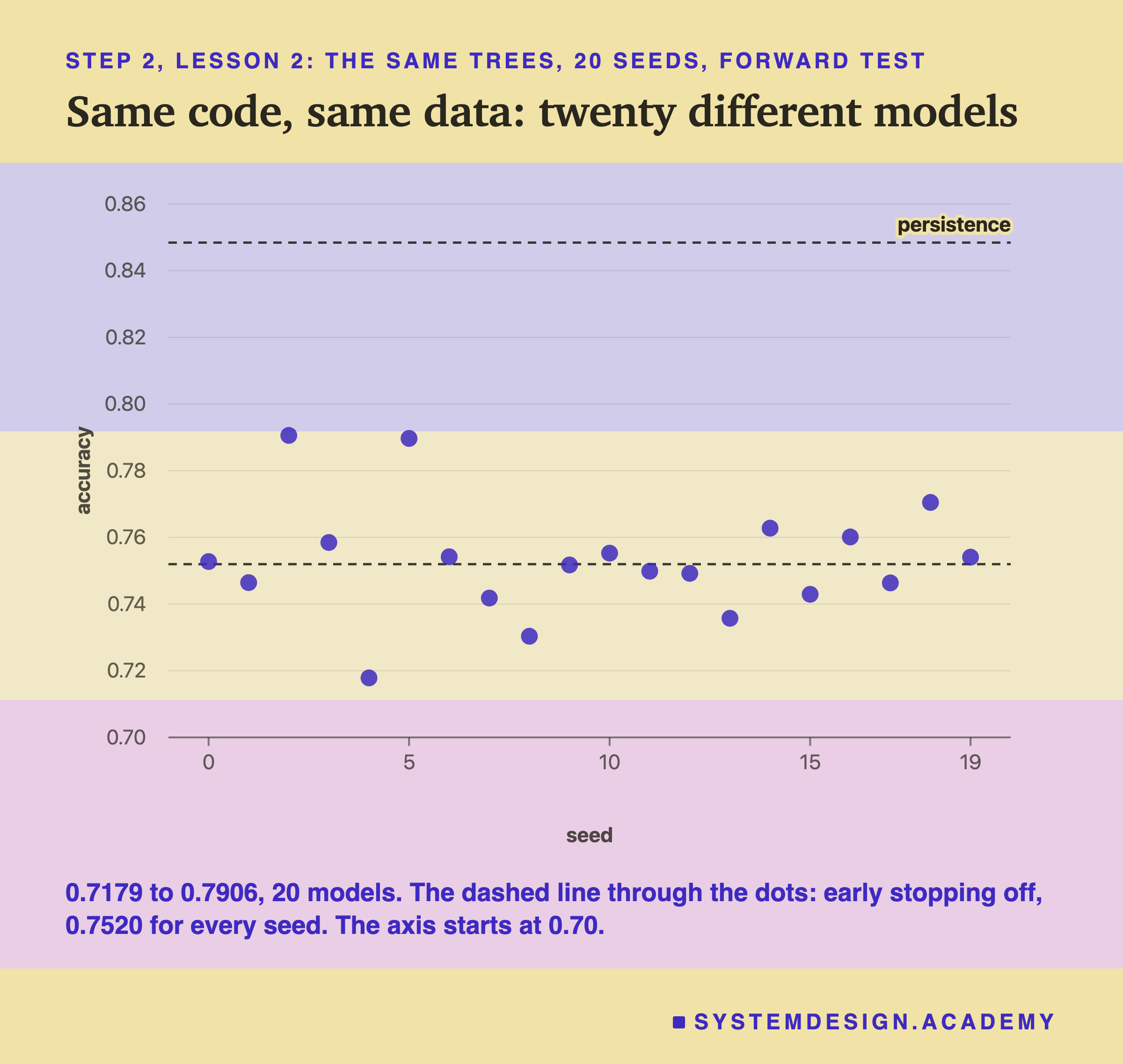
What went wrong, measured. The same boosted trees, the same code and the same data, trained 20 times with only the seed changed (the starting number for the program's random choices), gave 20 different models. On the future they scored from 0.7179 to 0.7906, a spread of 7.3 points, and two of them disagreed on up to 19.7% of the test rows. The cause was a default setting nobody wrote: above 10,000 rows, scikit-learn's boosted trees switch on early stopping, which sets aside a random tenth of the training rows, chosen by the seed. Every run built all 100 trees, so nothing ever stopped early; the seed only changed which tenth was left out. With early stopping switched off, every seed gave one model, 0.7520.

What saw it. Running more than one seed. One run shows one number and hides the spread completely. After the results, lesson 2's report rebuilt each seed's hidden slice and showed that, in all 20 of 20 seeds, the default model gives the same answer on every test row as a model trained without early stopping on the 90% that was kept. Running the same seed 20 times gave one model, so the computer itself added no noise.

What the lesson could not show. Other kinds of model, such as neural networks, have other sources of randomness that this lab did not touch, and it never checked another library version or another machine. It also showed why one run is not enough to compare two models: 70 of the 190 pairs of seeds were more than 2 points apart with nothing changed at all.

What it is for. Before training, someone chooses settings, such as how fast the trees learn and how big they grow. Tuning tries many settings and keeps the one that scores best on a validation set, rows held back only for choosing. A separate test set is looked at once, at the end, to find out what the choice is worth.

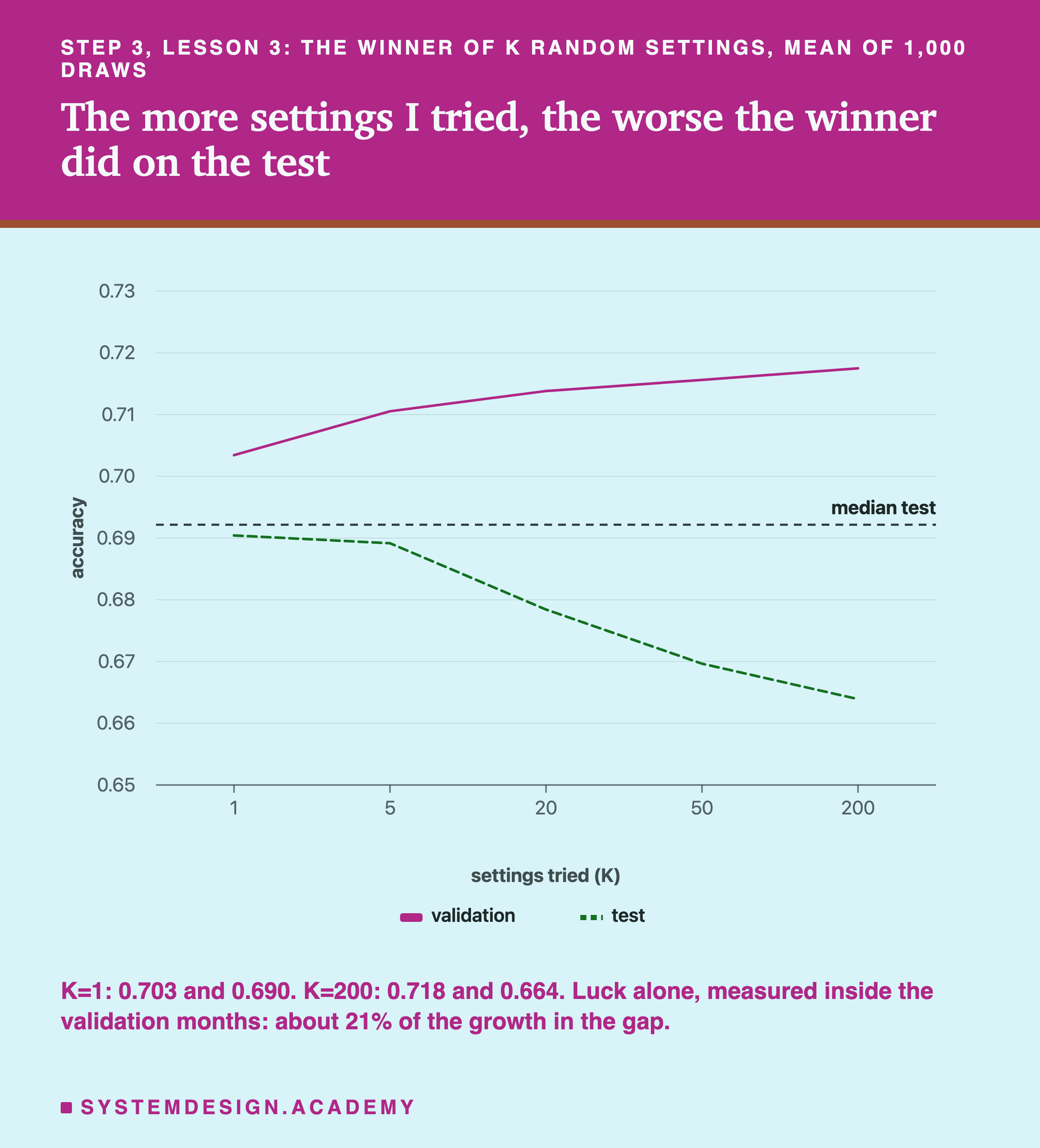
What went wrong, measured. I drew 200 random settings, kept the best on validation, and repeated the game 1,000 times for several sizes of search. Picking one setting at random gave 0.703 on validation and 0.690 on test. The best of 200 gave 0.718 and 0.664: its test score came 173rd of the 200. Trying more raised the score I could see and lowered the one I could not. The gap between them grew from 1.3 points with no choosing to 5.4 points at 200.

Here is the correction lesson 3 made after its review, and it matters. Most of that growth was not luck. A fair control, which split the validation months' own days into two halves, found that ordinary selection luck accounted for 0.86 of the 4.06 points of growth, about a fifth. The rest came from choosing on months that were unlike the months the model then served: the validation months, November 1997 to the first morning of June 1998, rewarded different settings from the test months, June to December. Lesson 3 also kept a limit on that control: neighbouring days are alike, so two halves made of mixed days are more alike than two truly independent samples, and the control may understate luck.

What saw it. Only the untouched test set. While choosing, nothing warned: the rank correlation between validation and test scores over all 200 settings was 0.03, almost no relation. The best setting on the test itself scored 0.750, and persistence still scored 0.848 on the same rows.

What the lesson could not show. Smarter search methods, a winner retrained on training and validation together, and data that does not drift, where luck might be most of the story.

What it is for. A pipeline that retrains a model must decide whether the new one, the challenger, replaces the live one, the champion. The rule that decides is the promotion gate, and it is only as good as what it demands.

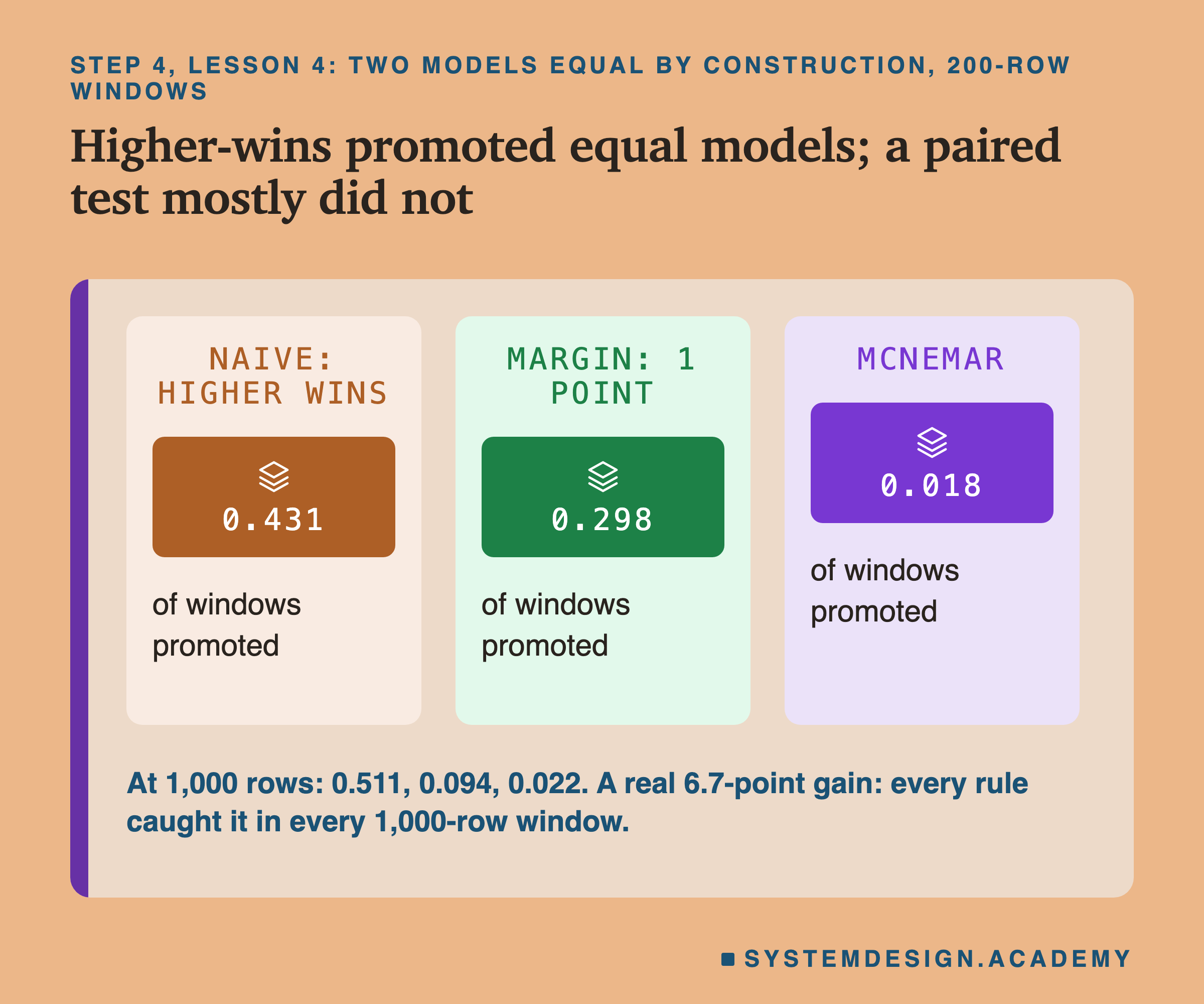
What went wrong, measured. I first planned pairs of seeds as models that are equally good. Lesson 4 found that they were not: on the whole test, the second seed of a pair was from 3.2 points worse to 7.2 points better, and 18 of the 20 pairs clearly differed. That is lesson 2 again, showing up at the gate: a retrain with a new seed is a different model. So a follow-up built models equal by construction, by tossing a coin on every row to decide which model got which outcome. On those, the rule "promote if the new score is higher" promoted the challenger in 0.43 of 200-row windows and 0.51 of 1,000-row windows: a coin flip at every size. A fixed 1-point margin promoted it in 0.30 of 200-row windows and 0.09 of 1,000-row windows, so its safety depended on the window. And checking again and again made things worse: over 45 checks as rows arrived, McNemar's test promoted 6 of the 20 equal challengers at some check, against 2 with one check at the end.

What saw it. The coin swap itself, which showed that higher-wins and a fixed margin promote equal models far too often. McNemar's test, which counts only the rows where exactly one of the two models was right and asks whether that split is too uneven for coin flips, promoted in 0.018 and 0.022 of windows. Lesson 4 is careful about what that shows, and so am I: under the swap, McNemar holding near its line is what the maths requires, because the swap builds exactly the coin-flip assumption the test rests on. The new evidence is about the other two rules. McNemar still caught a real 6.7-point gain in every 1,000-row window, though only in 0.578 of 200-row windows.

What the lesson could not show. The coin swap also broke the link between neighbouring half-hours, so it cannot say whether real windows of alike rows fool the test. And there was no pair with a small real gain, so how many rows a 1-point gain needs is unknown here.

What it is for. A model that passed the gate on stored rows can still be worse on today's rows. A canary sends a share of live rows to the new model; shadow runs the new model silently on every row next to the old one. Both look for a regression, a new version that is worse.

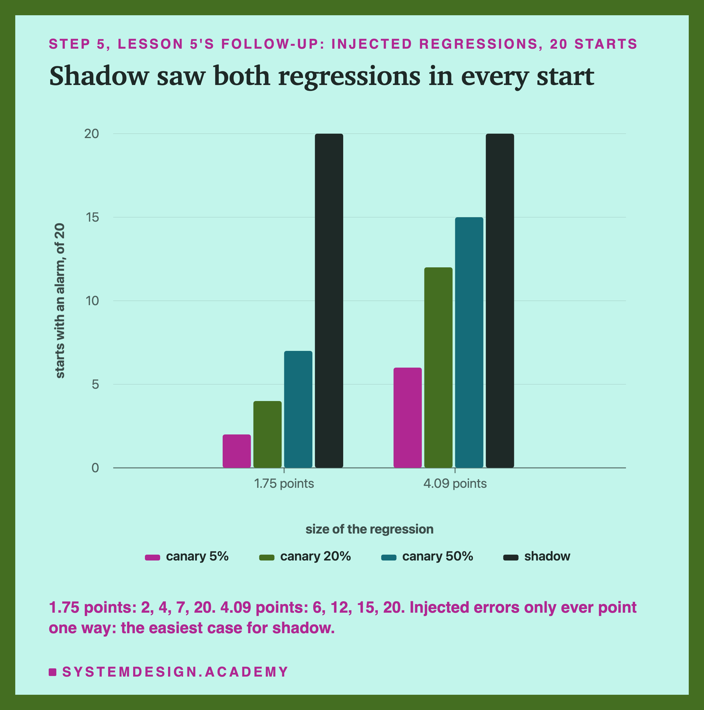
What went wrong, measured. First, my own design went wrong twice, and lesson 5 kept both on the record. The planned "small regression", the trees without two inputs, was in fact 0.61 points better than the champion. And the planned equal challenger was the champion itself, which can never disagree with itself, so shadow could not have raised any alarm on it. A follow-up, designed after the results, replaced both. On a known regression of 4.09 points, a canary sending 20% of the rows raised the alarm in only 12 of 20 starting points in 2,000 half-hours; at 5% in 6. On 1.75 points, the 20% canary caught 4 of 20. And checking the canary after every half-hour, instead of once at the end, raised its false alarms on equal models from 1.1% to 9.8% of runs.

What saw it. Shadow, because it compares both models on the same rows: it caught both injected regressions in all 20 starts, the 4.09-point one after a median of 241.5 half-hours. On the real regression of the main run, the logistic model, shadow raised the alarm first in every start where a 20% canary also did, 15 of 15, and alone in 3 more.

What the lesson could not show. The injected errors only ever turned right answers wrong, which is the easiest case for a paired test; the real regression came in runs, with a correlation of 0.57 between neighbouring rows against 0.01 for the injected errors. There was no real traffic, one row per half-hour, and nothing about how users react to new answers, which only a canary can see.

What it is for. A model learns from the past and then answers a future that drifts away from it. A retrain policy decides when to train it again: on a schedule, or when a measurement says it got worse, which is called a trigger.

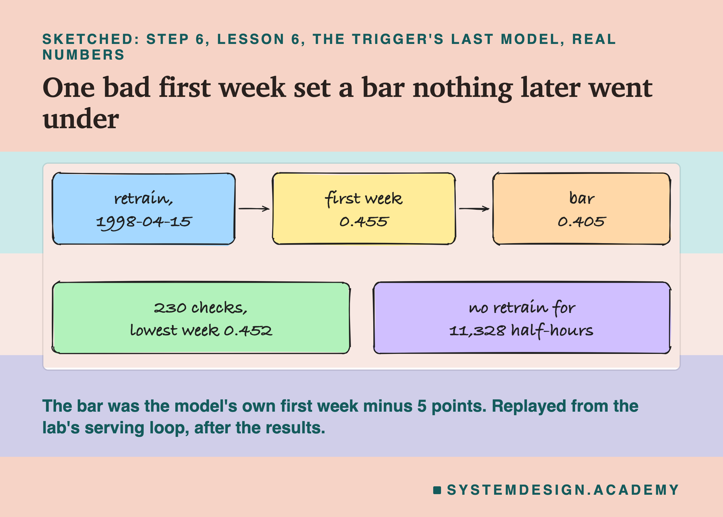
What went wrong, measured. Over 22,656 served half-hours, never retraining scored 0.6610, retraining every 28 days 0.7516 with 16 retrains, and every week 0.7636 with 67. The trigger, which retrained when the last week fell 5 points below the model's own first week, scored only 0.6812 with 8 retrains. The report replayed its log and found why: the last model it trained, on 15 April 1998, had a first week of 0.455, so its bar was 0.405. In 230 daily checks its weekly accuracy never went below 0.452, so it served 11,328 half-hours, half the run, without a retrain. The rule was anchored to one bad week.

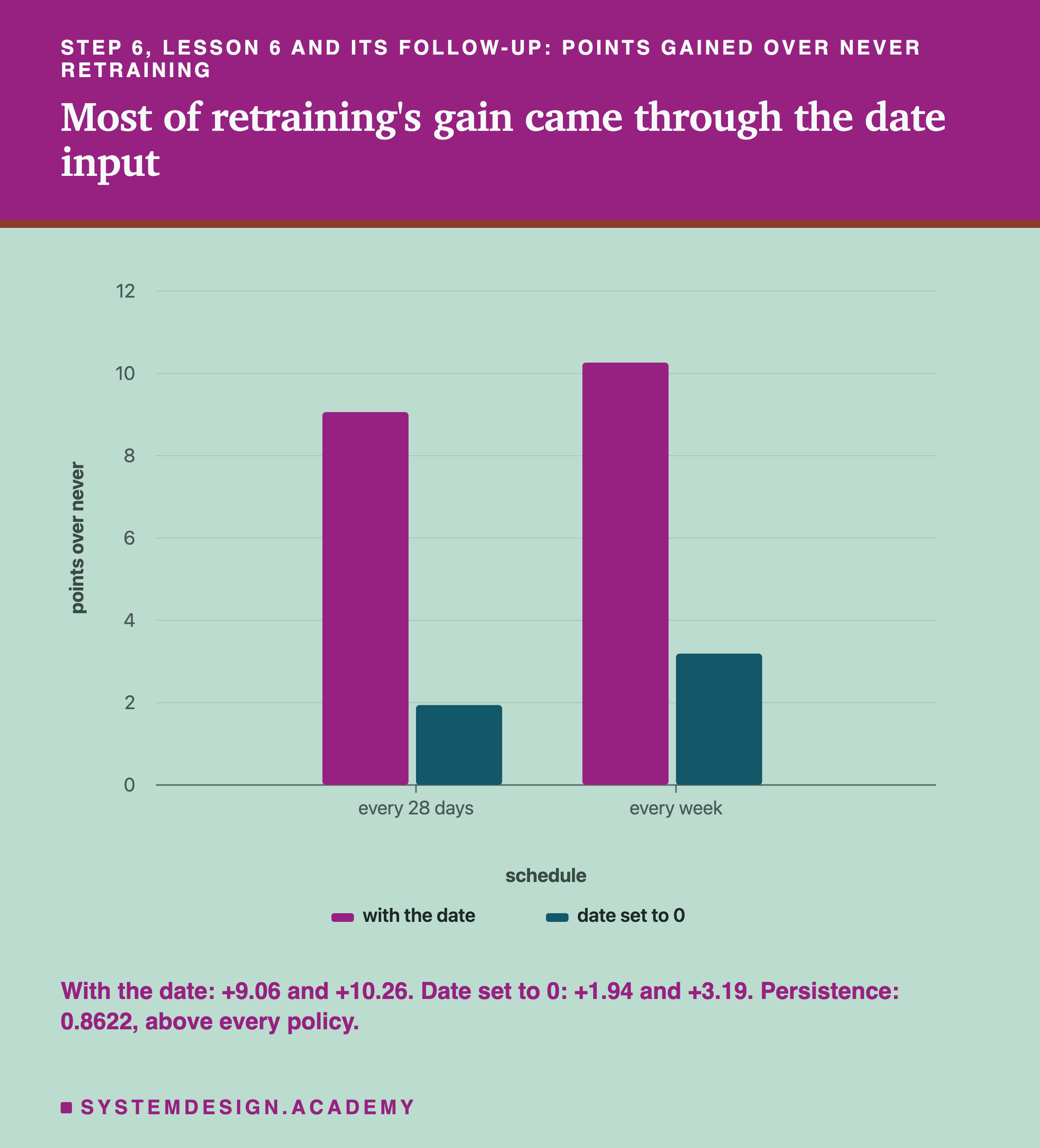
The second finding came from a follow-up and changed how I read the first. Most of what retraining bought came through one input, date. Every served half-hour had a date larger than any the first model had learned from, and the frozen model gave the same answer on 100.0% of rows when its dates were replaced by its last training date. With the date input set to 0, monthly and weekly retraining gained only 1.94 and 3.19 points over never, instead of 9.06 and 10.26. And persistence, 0.8622 on the same rows, stayed above every policy.

What saw it. Nothing running at the time. The trigger checked every day and saw nothing wrong by its own rule; only a replay of its log after the run showed the anchored bar. A fixed floor, retraining whenever a week fell below 0.65, 0.70 or 0.75, avoided the anchoring in a follow-up (0.7578, 0.7518 and 0.7656), but I chose those levels after seeing the results.

What it is for. Between the data and the model sit other parts of a pipeline: an input stored in a cache and reused instead of computed again, or a saved file such as a scaler, which rescales the inputs before the model reads them. They must stay in step with the model.

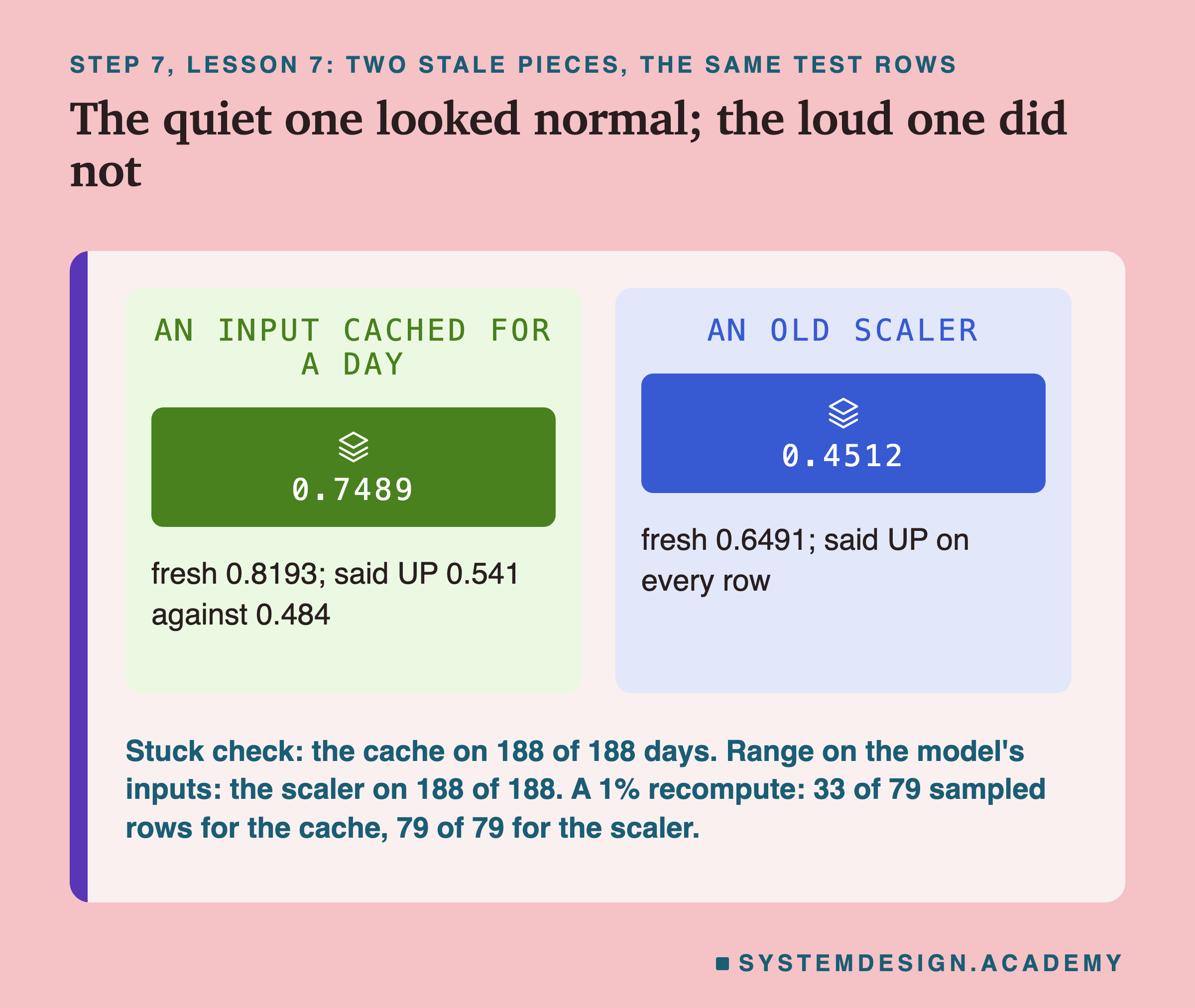
What went wrong, measured. The previous half-hour's label, cached once a day instead of computed each half-hour, cut the trees plus lag from 0.8193 to 0.7489, a loss of 7.04 points. Lesson 7's review corrected how I first read that: 0.7489 is a tie with the trees that never had the lag at all, 0.7527 (McNemar p 0.353), not worse than them. The day-old lag simply threw away everything the lag had added. And from outside it looked normal: the share of answers that were UP moved only from 0.484 to 0.541. The second stale piece was loud. The logistic model served through a scaler left over from the first 10% of the data scored 0.4512 and said UP on every row, because the old scaler turned the growing date into a number more than 200 spreads above anything the model had seen.

What saw it. A different check for each piece, both chosen after the results. A stuck check, which fires when an input that should move holds one value all day, caught the cache on 188 of 188 test days, and fired on 1 day with the fresh input. A range check on the numbers the model actually received caught the old scaler on all 188 days, while the same check on the raw inputs could not see it at all. As first written that range check had no margin, and lesson 7 found it needs one: with the date left out and a margin of 0.1 spreads it fired on 0.037 of days, and with any sensible margin only the date tripped it, every day. The daily share of UP answers missed the old scaler completely, because on training days the logistic model had already said DOWN on every row on 110 days and UP on every row on 2. Recomputing 1% of served inputs from scratch caught both: 33 of 79 sampled rows for the cache, 79 of 79 for the scaler.

What the lesson could not show. Both faults were built on purpose, one input and one file, so this is a demonstration of what each check can see, not a fair trial of the checks.

What it is for. On a bad morning, a team goes back to the model that worked. That needs either the saved model file or a complete record of how it was made, its lineage, so it can be rebuilt exactly.

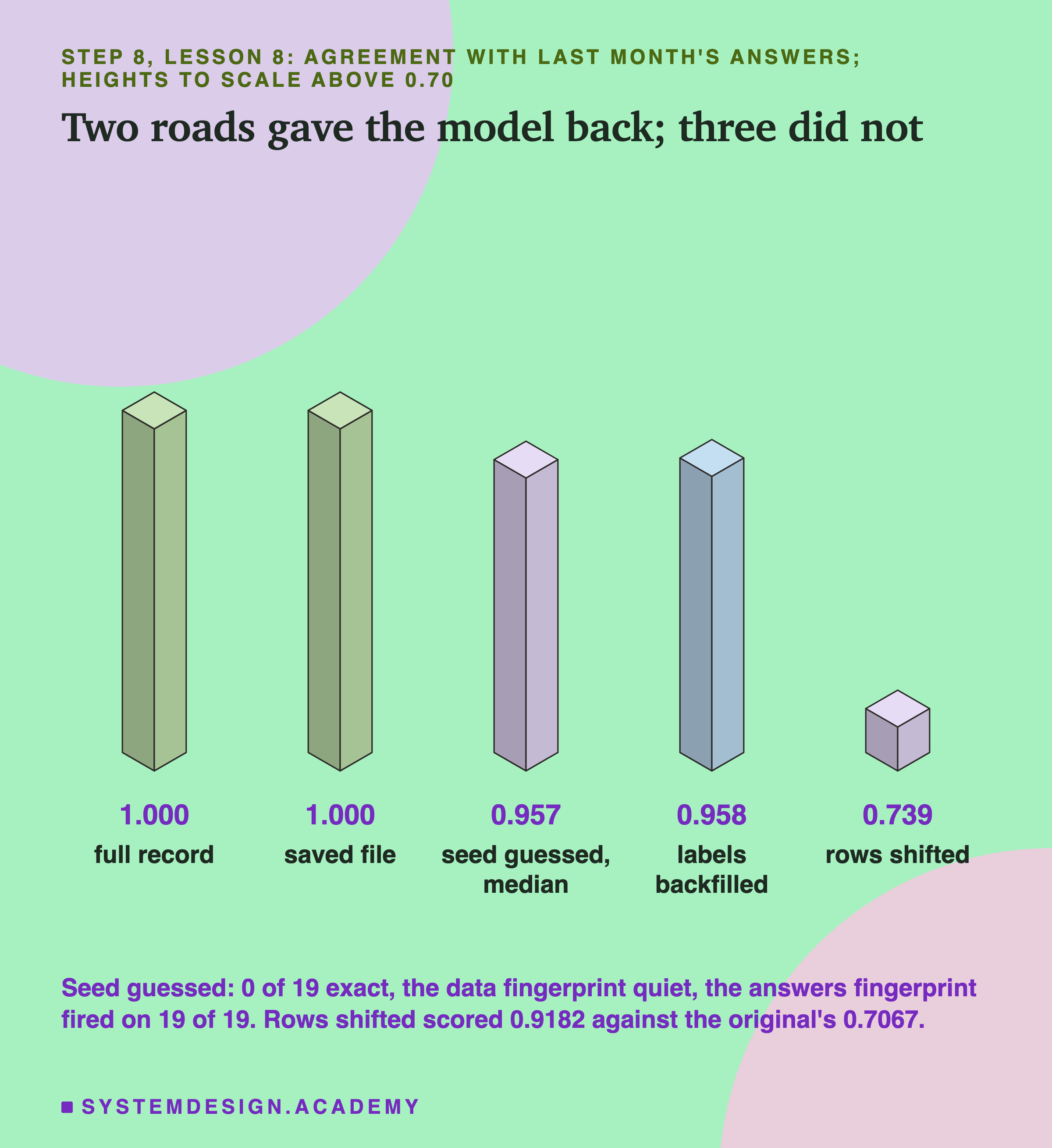
What went wrong, measured. Lesson 8 trained one model on rows 0 to 30,000 with seed 7 and tried five ways back. The full record and the saved file both gave the same answer on all 6,000 rows it had served. The other three did not. With the seed not written down, 19 guessed seeds agreed with it on 0.920 to 0.970 of rows, and none was exact. With 282 old labels corrected upstream, a rebuild agreed on 0.958. With the rows written as "the last 30,000" and read a month later, it agreed on only 0.739, and it scored 0.9182 on the served rows against the real model's 0.7067, because it had trained on those very rows. A wrong rebuild looked better than the truth.

What saw it. Two fingerprints in the record. A hash is a short code computed from exact numbers that changes if one number changes. The hash of the training rows fired for the corrected labels and the shifted rows. It stayed quiet for the missing seed, because the rows were right. Lesson 8's correction is the important one here: the missing seed is silent only to a record that describes the inputs. The hash of the model's answers on the stored month fired on all 19 guessed seeds.

What the lesson could not show. A change of library version, which it did not test. And the "month" was simulated: every rebuild ran seconds later, on the same machine, in the same program.

What it is for. A model can only learn from answers that have arrived, and a team can only score it on them. The label delay is how long the right answer takes to arrive. Here it decides both learning and knowing.

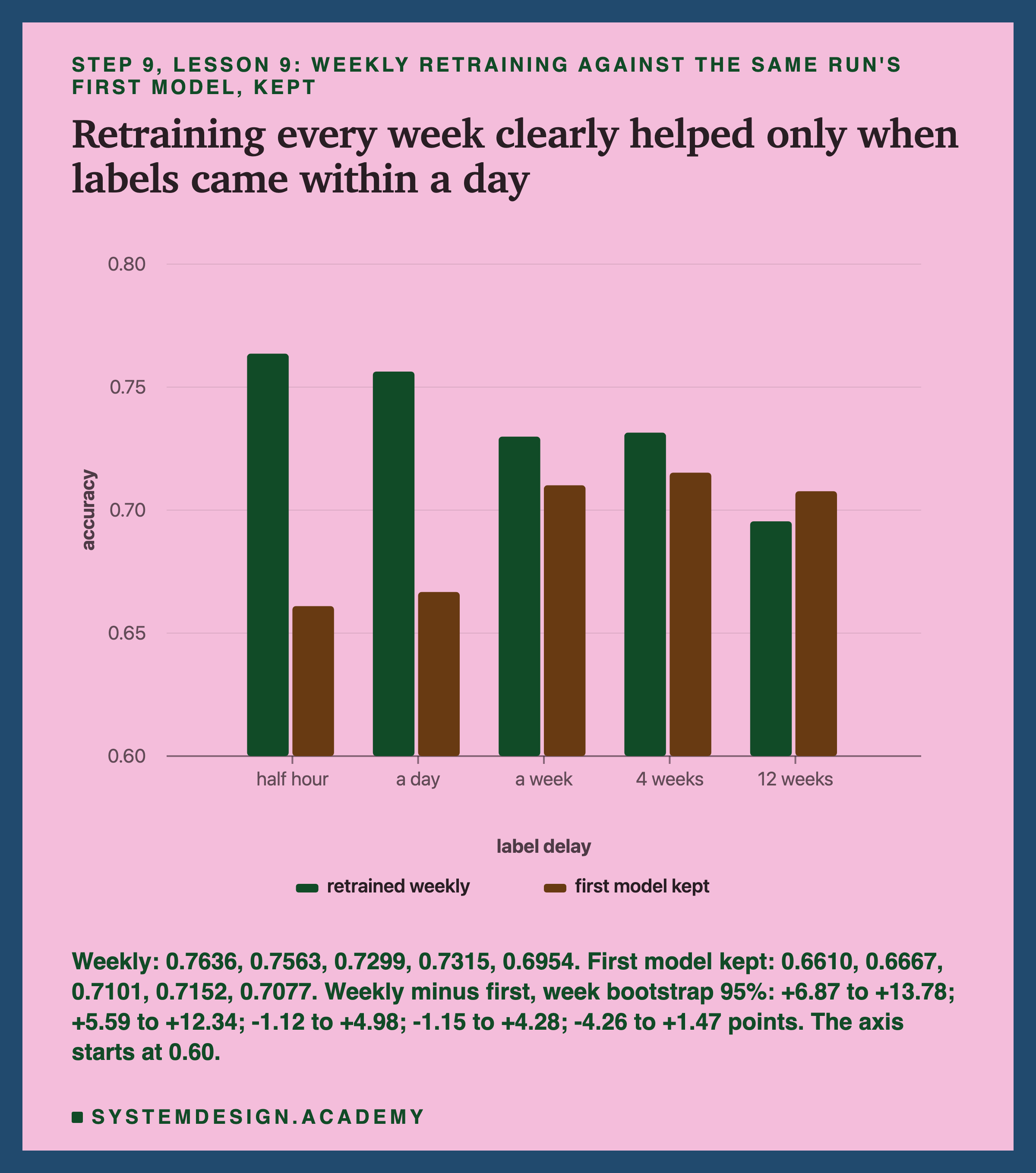
What went wrong, measured. Lesson 9 retrained the model every week while the labels arrived half an hour, a day, a week, four weeks or twelve weeks late. Accuracy went 0.7636, 0.7563, 0.7299, 0.7315 and 0.6954. Four weeks scoring above one week looks backwards, but the two differed by 36 rows out of 22,656 (McNemar p 0.59), and a bootstrap over whole weeks gave an interval of -2.38 to +2.72 points, so the order is noise. A day's cost, 0.73 points, also could not be told apart from chance.

Lesson 9's review changed the comparison with never retraining, and I use the corrected one. The 0.6610 "never" line from lesson 6 was a model trained with fresh labels, which a team with late labels could never have had. The fair comparison for each delay is that run's own first model, kept forever: 0.6610, 0.6667, 0.7101, 0.7152 and 0.7077 for the five delays. Weekly retraining clearly helped only when the labels arrived within a day: +10.26 and +8.96 points, with week-bootstrap intervals of +6.87 to +13.78 and +5.59 to +12.34, both far above zero. At a week and at four weeks the small gains, +1.98 and +1.62, cannot be told apart from chance (-1.12 to +4.98 and -1.15 to +4.28). Twelve weeks late it scored lower than its first model kept, 0.6954 against 0.7077, and that gap also cannot be told apart from chance (-4.26 to +1.47). Lesson 9 added this bootstrap after its review.

What saw it. Nothing at the time. With labels twelve weeks late, a dashboard of weekly accuracy had nothing to show for the first 90 days, and then showed a fine week on 65 days when the real week was bad, and a bad week on 94 days when the real one was fine. Those two counts rest on levels, 0.65 and 0.70, that were chosen after lesson 6's results. A signal that needs no labels, how far the share of UP answers sat from training's, moved partly with weekly accuracy (a rank correlation of -0.60); the model's own confidence did not (-0.08).

The last step feeds the first, and on this data it does so in a very plain way. The best rule of the whole chapter, persistence, uses exactly one thing: the previous half-hour's label. It scored 0.8484 on lesson 1's test and 0.8622 on the served half of lessons 6 and 9, above every trained model and every retraining policy.

That rule only exists because the labels come back in half an hour. With a delay of a day, persistence would have to repeat yesterday's label at the same half-hour, a weaker rule that lesson 1 measured at 0.6741. With a delay of twelve weeks it would be almost meaningless. So the label delay of step 9 decides which baselines step 1 is allowed to use. A team that measures its baseline with labels it will not have in service is setting a bar it cannot reach, which is a framing point lesson 1 made at its start: write down what is known when each guess is made.

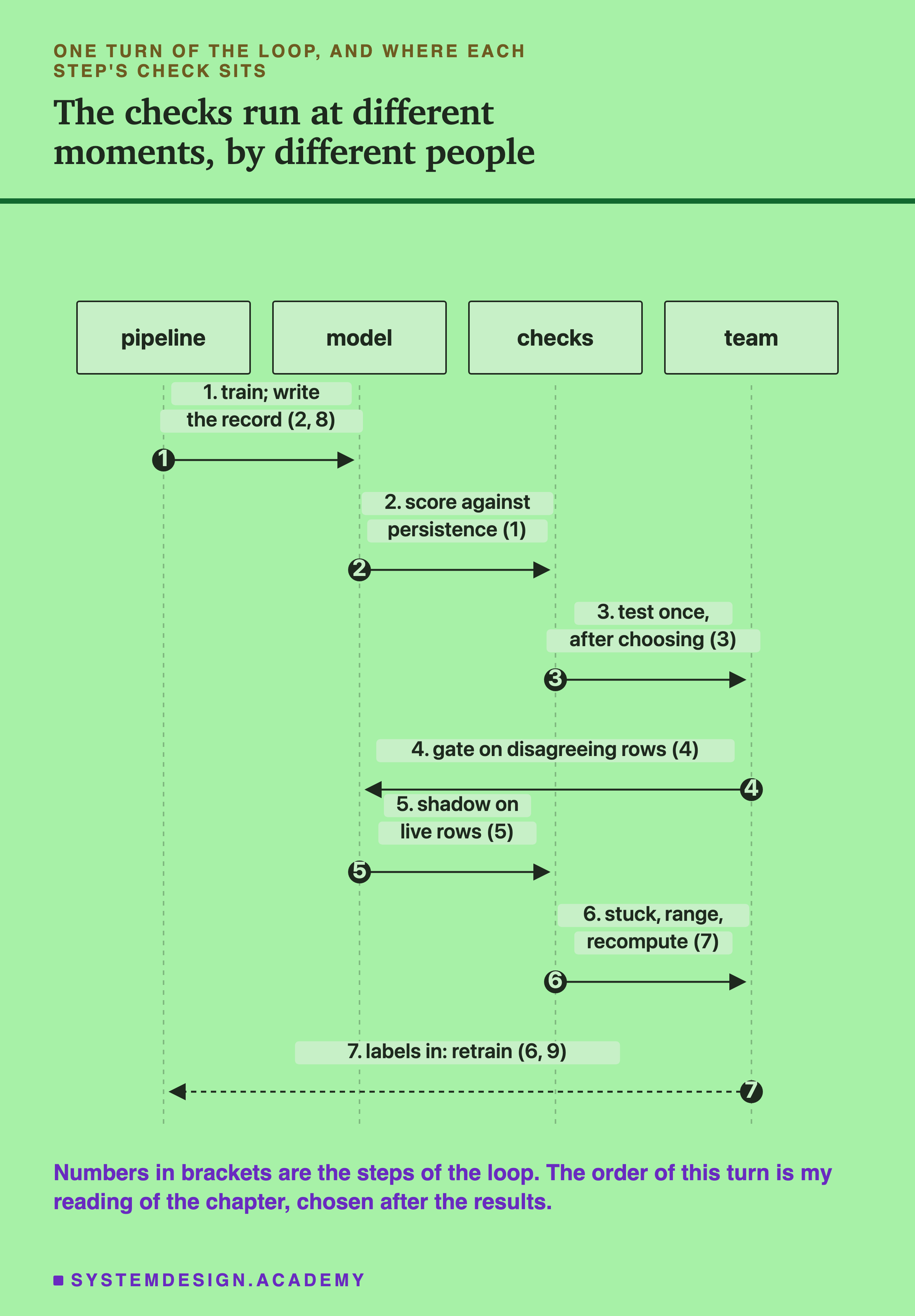
The sequence above places each step's check in one turn of the loop, as I read the chapter. The pipeline trains a model and writes its record, the record that steps 2 and 8 need. The model is scored against persistence. The chosen setting is tested once. The gate compares on the rows where the two models disagree. Shadow runs on live rows. The pipeline's pieces are checked for staleness. Then labels arrive, and the loop starts again with a retrain. The order is my reading, chosen after the results; the lessons ran one step at a time.

One more thing ties the turn together. Every check in it runs at a different moment, and usually belongs to a different person: the person who trains, the person who owns the gate, the person on call when something breaks. In my experience, which this chapter did not measure, the checks that nobody owns are the ones that stop being run.

After all nine results were in, I put each step's measured failure next to what saw it. Nothing in this table was measured for this lesson; it is read from the stored files.

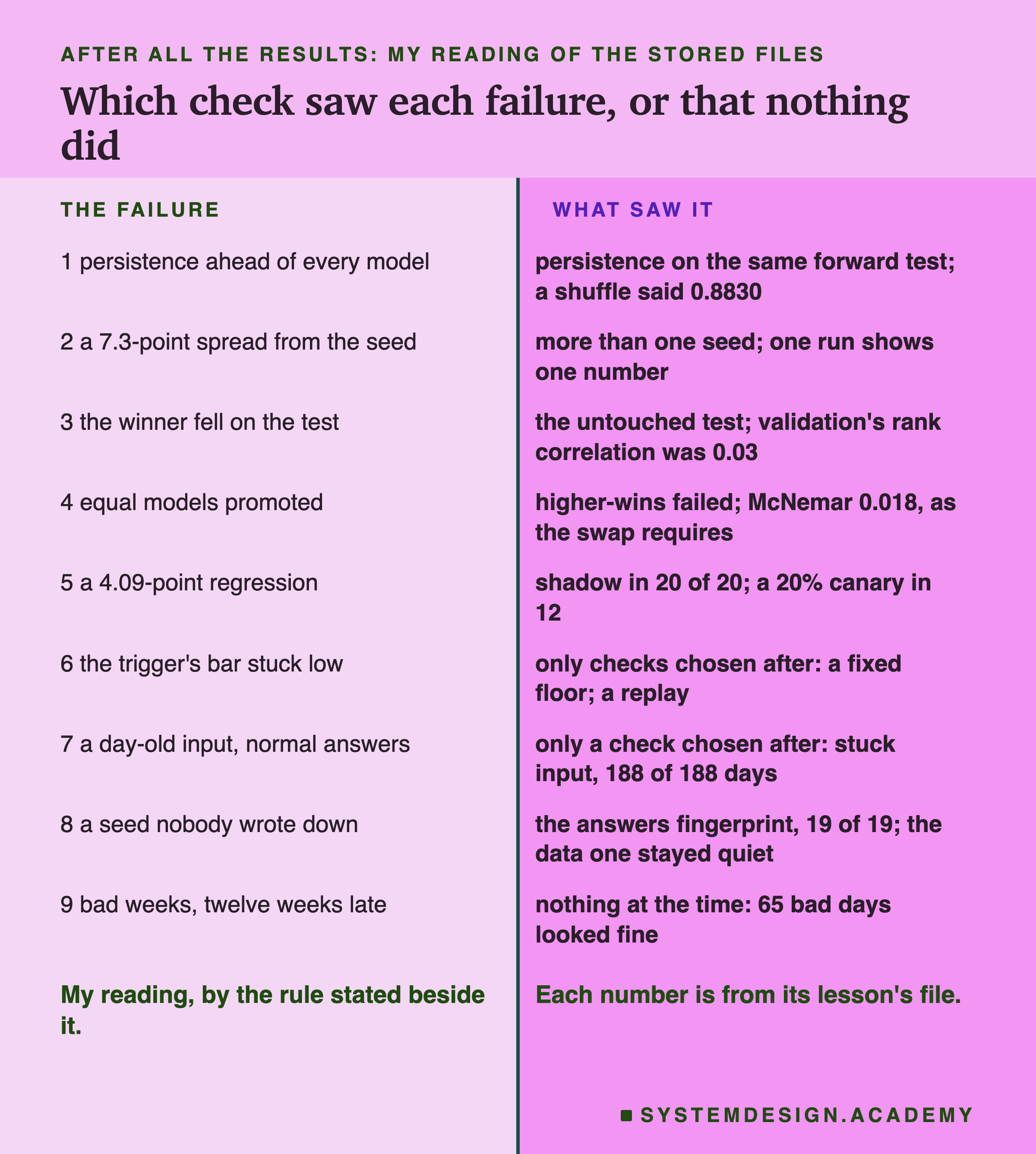
First, the rule I used for "seen", because the count that follows depends on it, and it is my reading, not a measurement. A failure counts as seen at the time if some check in the chapter fired on it clearly using only what the pipeline had at that moment: no replay of a log after the run, and no labels that had not yet arrived. I also note whether that check was written into the lab's design before the run, or chosen by me after the results. This is a different question from whether a failure was silent, which is about whether the answers looked normal. By that rule the nine rows fall into four kinds.

In the first kind, a check from the lab's own design saw the failure clearly: persistence scored on the same forward test (step 1), shadow on the same live rows (step 5) and the fingerprint of the model's answers (step 8). None of these needs anything exotic. Each is a few lines of code or a single extra number.

In the second kind, the check was also in the design, but it costs more than a single run: running more seeds (step 2), or keeping a test set that nobody chose with (step 3). These cost more training, and they are exactly the things that get skipped when a team is in a hurry. Step 4 belongs here too, with a caveat. The coin swap showed that higher-wins and a fixed margin promote equal models far too often; McNemar holding near its line under the swap is what the maths requires, not a test of McNemar on real windows of alike rows.

In the third kind, only a check I chose after the results saw it. For the trigger of step 6, that was a fixed floor, which retrained where the self-referenced bar did not, and a replay of the trigger's log, which showed the bar stuck at 0.405. For the day-old cache of step 7, it was a stuck-input check. I count those two alike, because both checks were written knowing what they had to catch.

A failure that no check sees in time is the most expensive kind, because nothing makes anyone look, and it can run for months. By the rule on the previous slide, the chapter had one that nothing saw at the time, and two that only checks I chose after the results saw. A fourth is easy to miss for a different reason.

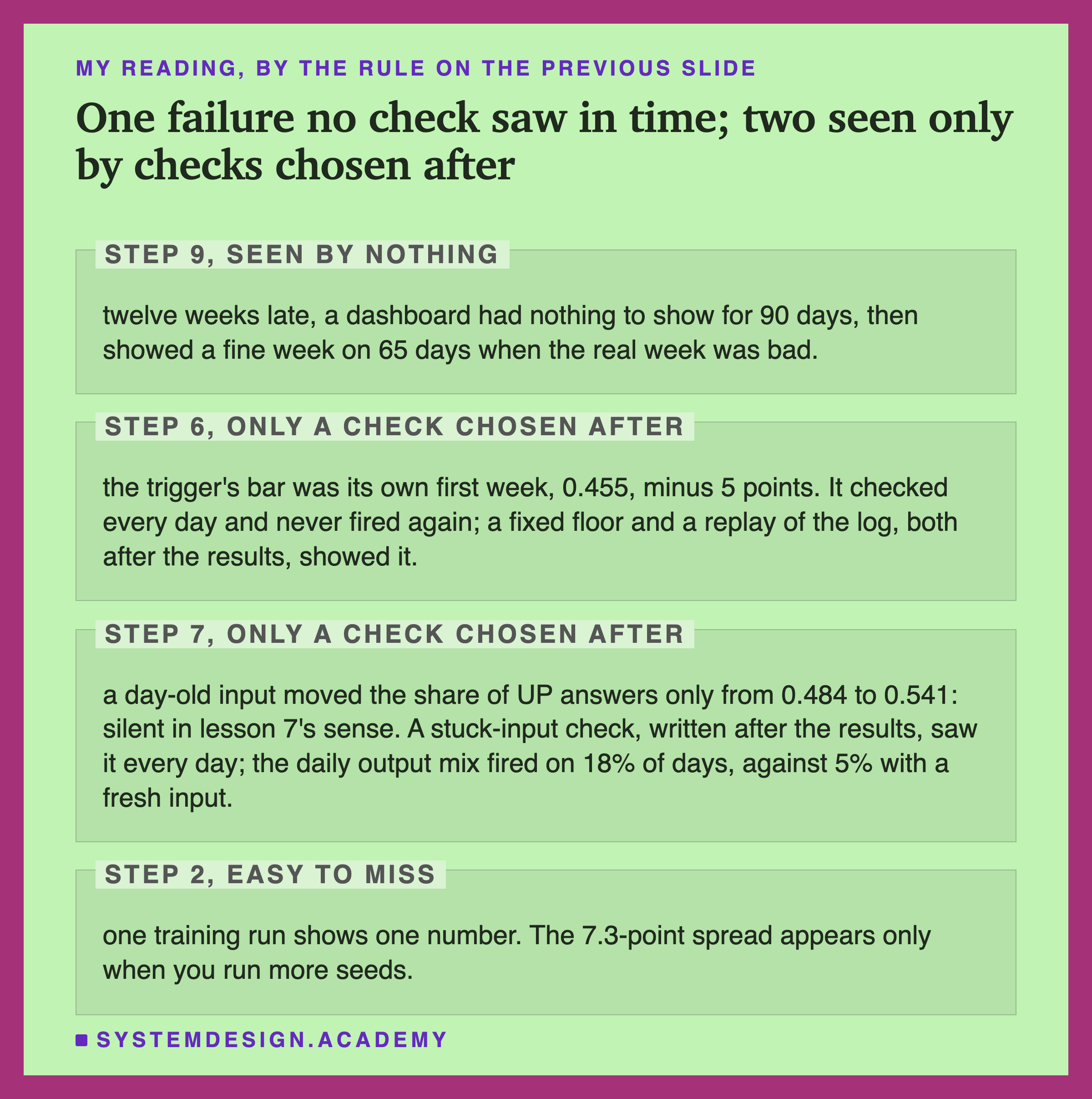
Seen only by a check chosen afterwards: the trigger. It did its job exactly as written. It measured a rolling week every day and compared it with a reference. The fault was in the reference: one bad week, 0.455, set the bar at 0.405. No alarm could ever say "the bar itself is wrong", because the bar was the thing the alarm used. What showed it was a comparison the trigger never made: a fixed floor, which lesson 6 tried in a follow-up with levels chosen after the results, and a replay of the log after the run.

Seen by nothing: the late dashboard. Every number it showed was correct about the week it described. The problem was which week that was: twelve weeks late, the newest complete week was 84 days old. A chart titled "accuracy, last 7 days" that shows a week from three months ago is not wrong about the past; it is wrong about now.

Seen only by a check chosen afterwards: the cached input. This one is also silent in lesson 7's sense: a day-old lag cost 7.04 points while the share of UP answers moved from 0.484 to 0.541, a gap that hides inside the ordinary swings of the season. The output checks fired on 18% of days against 5% with a fresh input, far too often on a healthy model to act on. Only the stuck check saw it every day, and I wrote that check knowing the result.

Easy to miss: the seed. Lesson 2's design ran 20 seeds, so the lab saw it. But one training run prints one number. The 7.3-point spread of step 2 only exists for someone who runs the same code more than once.

Some findings did not belong to one step. They came back in lesson after lesson, and they are the most useful things I learned from the chapter as a whole.

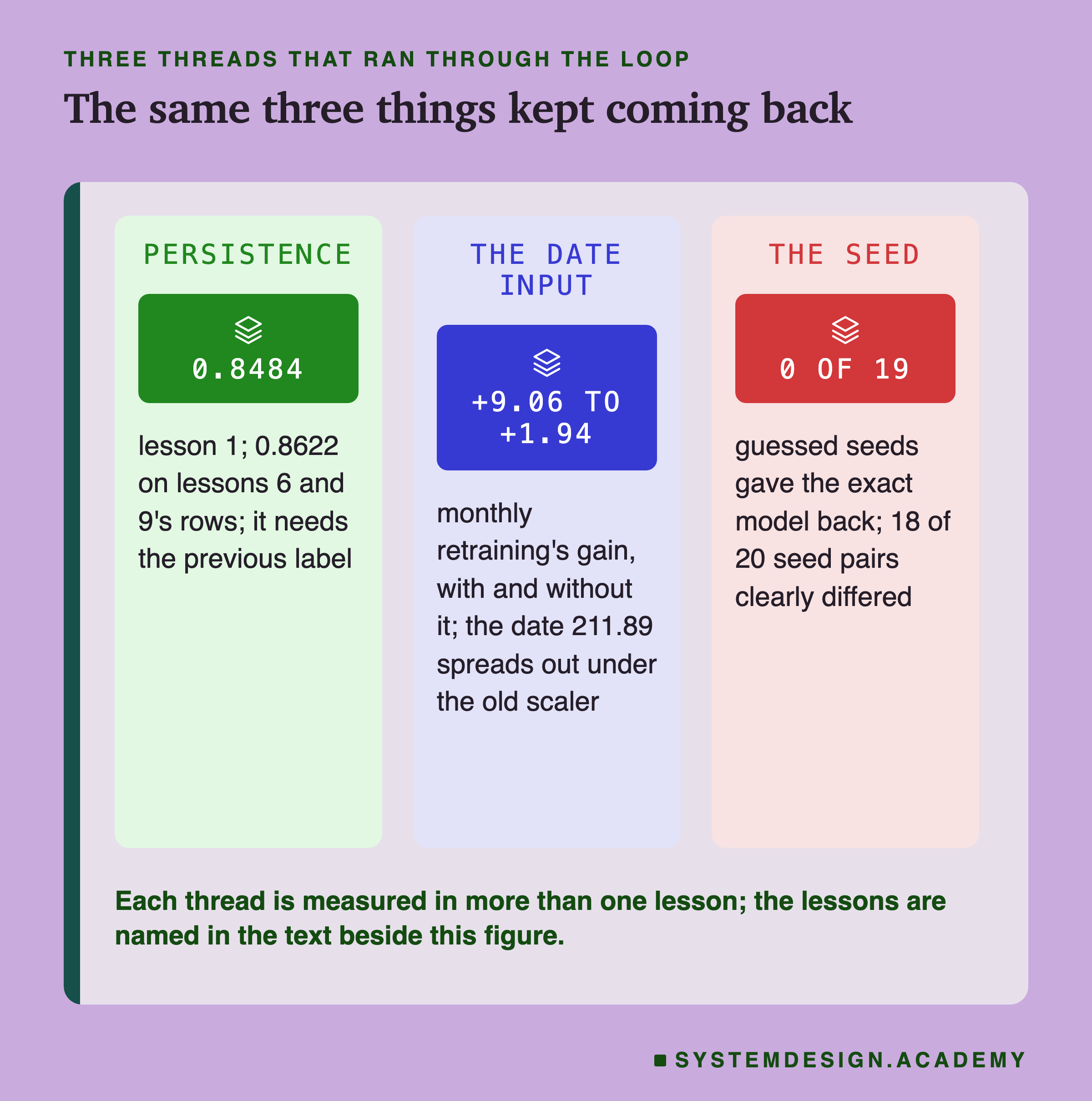
Persistence. A rule that learns nothing beat every trained model in lesson 1 (0.8484), stayed far above the best tuned setting in lesson 3 (0.848 against 0.750), stayed above every retraining policy in lesson 6 (0.8622) and needed labels half an hour old in lesson 9. On data whose labels repeat, the question "does this model beat persistence?" came before every other question, and the answer here was no.

The date input. An input that only says when did damage in two lessons and mattered in a third. In lesson 6 the frozen model treated every served half-hour as the last day of its training. Monthly retraining gained 9.06 points over never retraining with the date and 1.94 with the date set to 0, so about 7.1 of those points are tied to the date; lesson 6 calls its account of why, that retraining moved the model's idea of "latest" forward, its interpretation. In lesson 7 an old scaler turned the same date into a number more than 200 spreads out, and the model said UP on every row. In lesson 9 the date added 1.09 points with fresh labels (0.7636 against 0.7527) and almost nothing twelve weeks late (0.6954 against 0.6962); lesson 9 found that its first, unfair baseline, not the date, had decided how much late retraining appeared to help. Before measuring anything about time, find the inputs that only say when.

The seed. Randomness hidden in a default setting made 20 models from one piece of code in lesson 2, made pairs of seeds genuinely different models at lesson 4's gate (18 of 20 clearly differed), and made a lost seed impossible to recover in lesson 8 (0 exact of 19 guesses). Write it down, and never compare two models on one run each.

Every lesson in this chapter was reviewed before it went live, and several of them changed what they said after a review or a follow-up. The wrap has to agree with what each lesson finally says, so here are the corrections in one place.

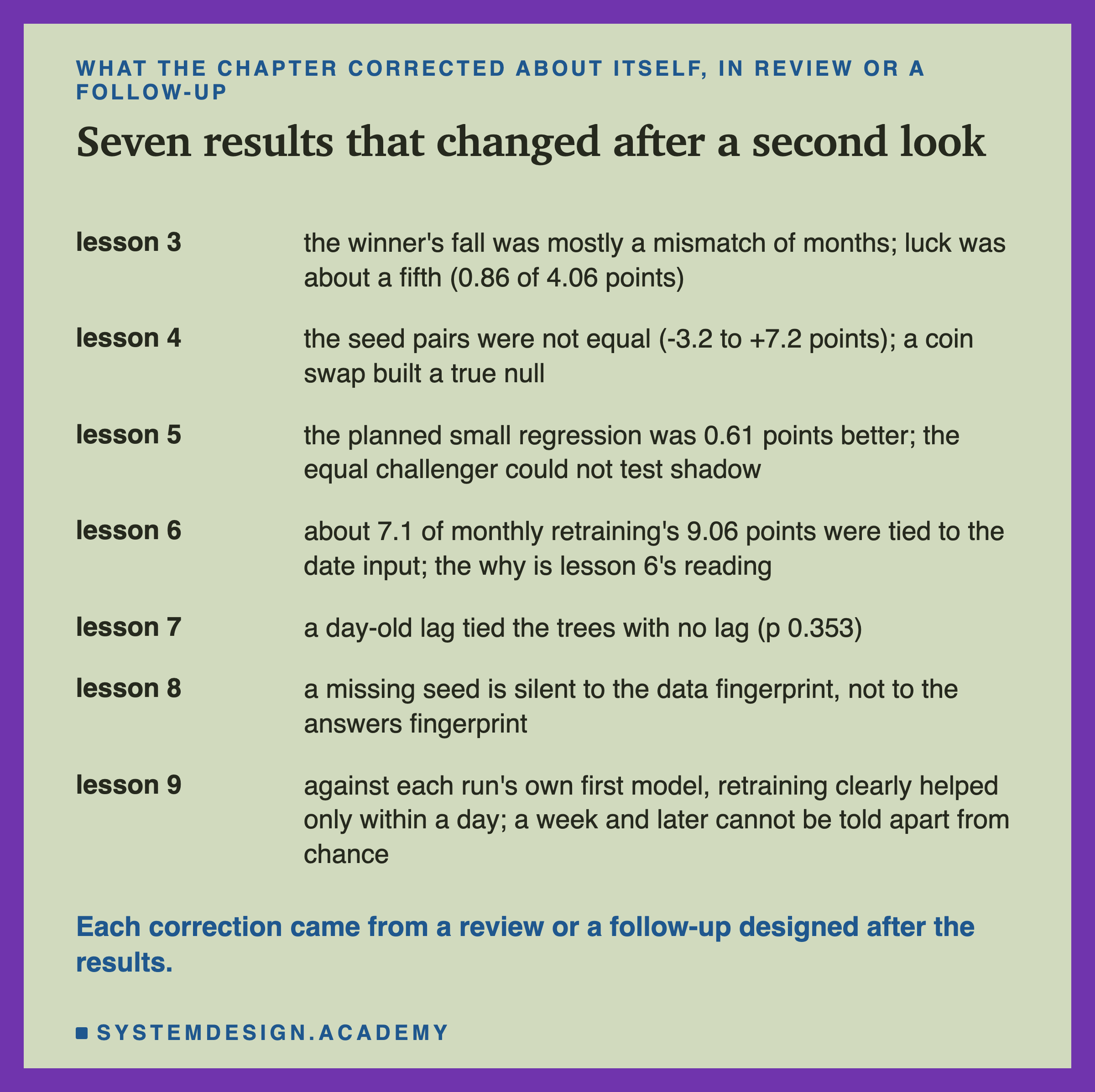
Lesson 3 first read its growing gap as the winner's curse, selection luck. A fairer control found luck was about a fifth of the growth, 0.86 of 4.06 points, and most of it came from choosing on months unlike the months served. Lesson 4 designed its "null" pairs as equal models, and they were not; a coin swap built a true null. Lesson 5's planned small regression was 0.61 points better, and its equal challenger could not test shadow; a follow-up replaced both. Lesson 6 found that about 7.1 of monthly retraining's 9.06 points were tied to the date input, and labelled its account of why as its interpretation. Lesson 7 first called the day-old cache worse than no lag at all; it was a tie, p 0.353. Lesson 8 first called the missing seed silent; it is silent to the data fingerprint and caught by the answers fingerprint every time. Lesson 9 first compared late retraining with a frozen model that had fresh labels; against each run's own first model, retraining clearly helped only within a day, and from a week on the difference could not be told apart from chance.

I include this slide because it is the pattern, not the exception. Each correction came from asking a result one more question, usually one a reviewer asked. Several of the lessons' clean first readings were wrong in a way the first design could not see, and the fix was always another measurement, never a better sentence. That is a reason to treat every number in this chapter, including the corrected ones, as one careful reading of one dataset.

Here is the chapter as one page, one line per step, in the loop's order. Each line is one lesson's advice, and each has a measured failure behind it. The wording is mine.

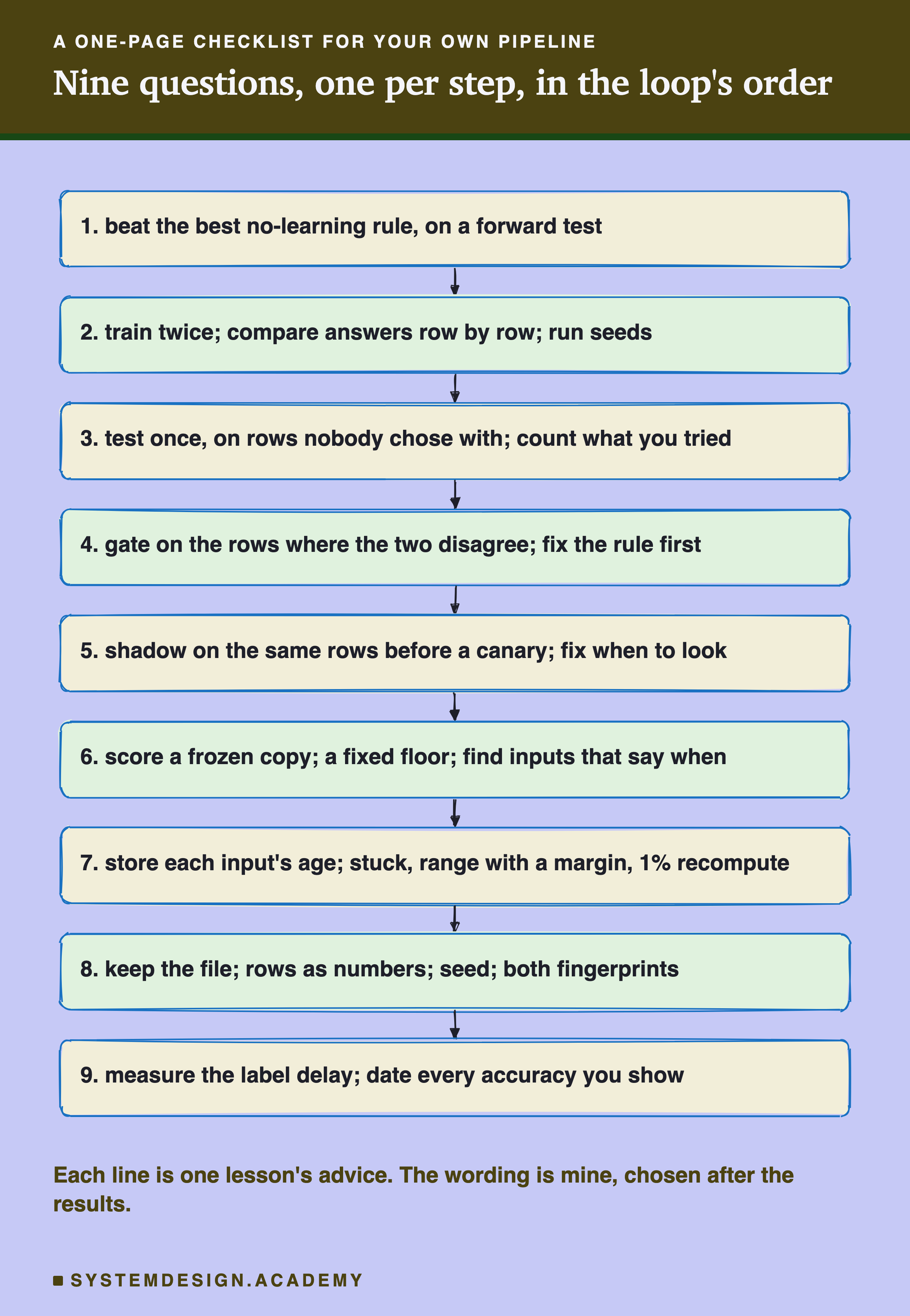
1. Beat the best no-learning rule, on a forward test. Score majority, persistence and a seasonal rule on the same future rows as the model. Here persistence won, 0.8484 against 0.8193.
2. Train twice and compare the answers row by row; then run several seeds. Here one piece of code gave 0.7179 to 0.7906.
3. Test once, on rows nobody chose with, and count what you tried. Report the winner's test score and K. Here the best of 200 was 0.718 on validation and 0.664 on test.
4. Gate on the rows where the two models disagree, with the rule written down first, and look once. Here higher-wins promoted equal models in 0.43 of windows, McNemar in 0.018.
5. Shadow on the same live rows before any canary, and decide in advance when to look. Here shadow caught a 4.09-point regression in 20 of 20 starts, a 20% canary in 12.
6. Score a frozen copy block by block, give any trigger a fixed floor, and find the inputs that only say when. Here a self-referenced trigger sat at 0.405 for half the run.
7. Store each cached value's age and each file's model version; run a stuck check, a range check with a margin on what the model receives, and a 1% fresh recompute. Here a day-old input cost 7.04 points and looked normal.

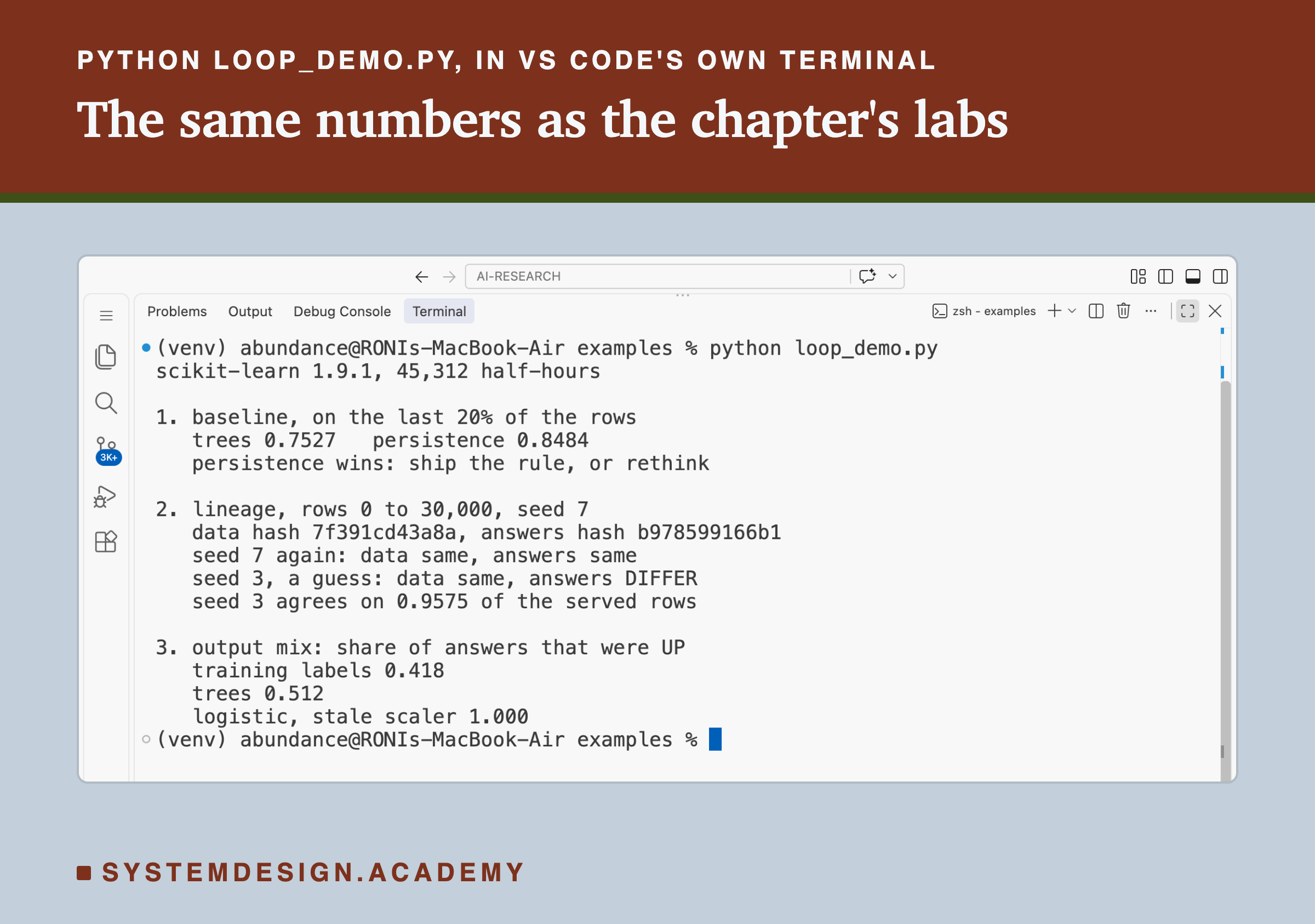
This script runs four of the loop's cheapest checks on Elec2: the baseline against persistence (step 1), the fingerprint of the training rows and of a model's answers, with one rebuild from the recorded seed and one from a guess (steps 2 and 8), and the output mix, the share of answers that were UP, for the trees and for the logistic model behind a stale scaler (a signal from lessons 7 and 9). It trains five small models and does not need a GPU.

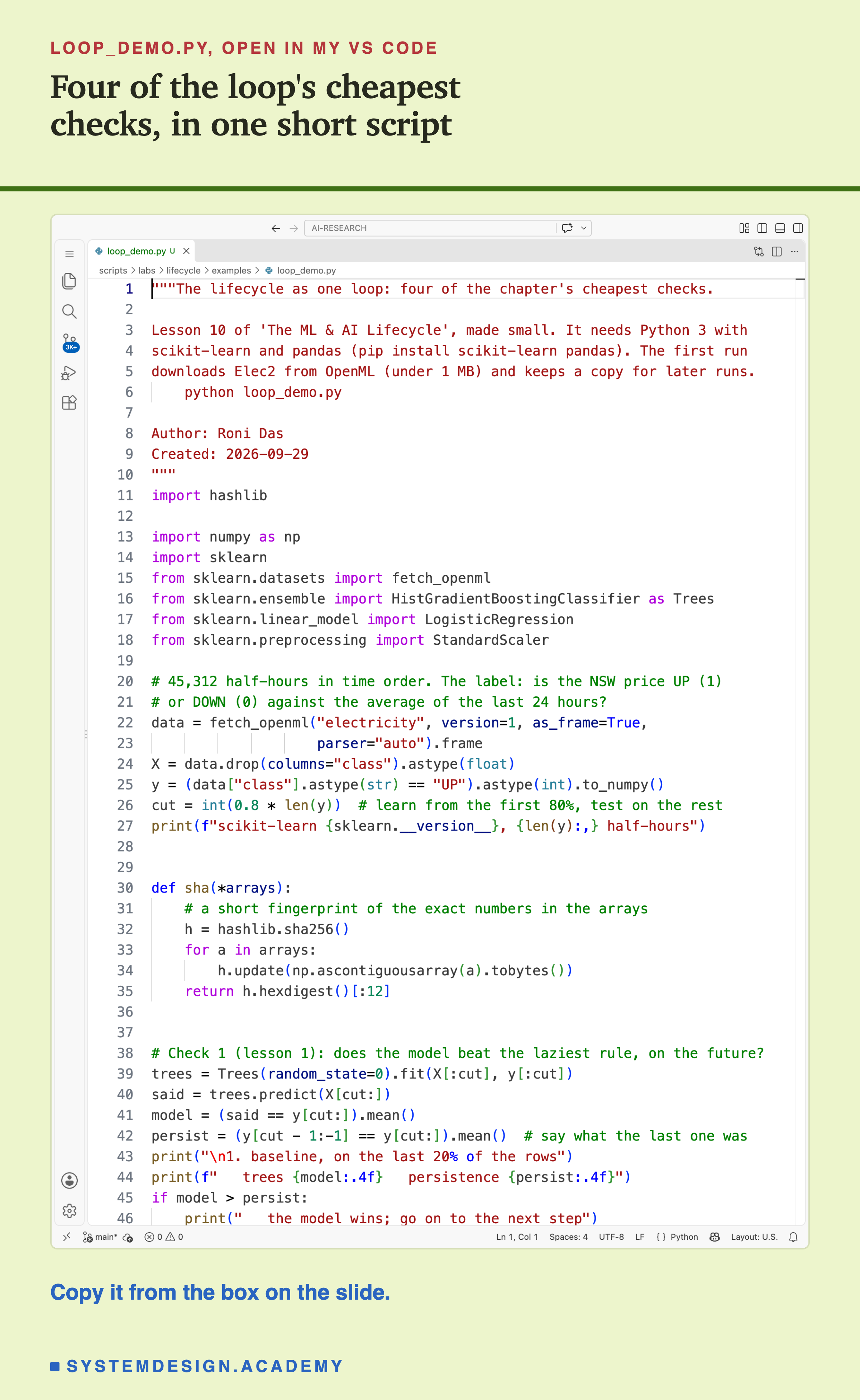
Before you run this lab. You need Python 3 and two libraries: pip install scikit-learn pandas. scikit-learn holds the models, the scaler and the download, and brings NumPy with it; pandas holds the table; hashlib comes with Python. The first run downloads Elec2 from OpenML, a free public website of datasets for machine learning (under 1 MB compressed), so it needs an internet connection once; scikit-learn keeps a copy in a folder in your home directory (scikit_learn_data) for later runs. I ran it with scikit-learn 1.9.1 on a Mac. scikit-learn runs the same way on Windows and Linux, but I have not checked the numbers there, and another version of scikit-learn may give different models and different fingerprints, which is lesson 8's point; that is why the first line printed is the version.

"""The lifecycle as one loop: four of the chapter's cheapest checks.

Lesson 10 of 'The ML & AI Lifecycle', made small. It needs Python 3 with
scikit-learn and pandas (pip install scikit-learn pandas). The first run
downloads Elec2 from OpenML (under 1 MB) and keeps a copy for later runs.
    python loop_demo.py

Author: Roni Das
Created: 2026-09-29
"""
import hashlib

import numpy as np
import sklearn
from sklearn.datasets import fetch_openml
from sklearn.ensemble import HistGradientBoostingClassifier as Trees
from sklearn.linear_model import LogisticRegression
from sklearn.preprocessing import StandardScaler

# 45,312 half-hours in time order. The label: is the NSW price UP (1)
# or DOWN (0) against the average of the last 24 hours?
data = fetch_openml("electricity", version=1, as_frame=True,
                    parser="auto").frame
X = data.drop(columns="class").astype(float)
y = (data["class"].astype(str) == "UP").astype(int).to_numpy()
cut = int(0.8 * len(y))  # learn from the first 80%, test on the rest
print(f"scikit-learn {sklearn.__version__}, {len(y):,} half-hours")


def sha(*arrays):
    # a short fingerprint of the exact numbers in the arrays
    h = hashlib.sha256()
    for a in arrays:
        h.update(np.ascontiguousarray(a).tobytes())
    return h.hexdigest()[:12]


# Check 1 (lesson 1): does the model beat the laziest rule, on the future?
trees = Trees(random_state=0).fit(X[:cut], y[:cut])
said = trees.predict(X[cut:])
model = (said == y[cut:]).mean()
persist = (y[cut - 1:-1] == y[cut:]).mean()  # say what the last one was
print("\n1. baseline, on the last 20% of the rows")
print(f"   trees {model:.4f}   persistence {persist:.4f}")
if model > persist:
    print("   the model wins; go on to the next step")
else:
    print("   persistence wins: ship the rule, or rethink")

# Checks 2 and 3 (lessons 2 and 8): fingerprint the training rows and
# the answers, then rebuild: once with the seed, once with a guess.
rows, month = slice(0, 30000), slice(30000, 36000)
first = Trees(random_state=7).fit(X[rows], y[rows])
served = first.predict(X[month])
data_hash = sha(X[rows].to_numpy(), y[rows])
answers_hash = sha(served)
print("\n2. lineage, rows 0 to 30,000, seed 7")
print(f"   data hash {data_hash}, answers hash {answers_hash}")
for seed, name in ((7, "seed 7 again"), (3, "seed 3, a guess")):
    again = Trees(random_state=seed).fit(X[rows], y[rows])
    answers = again.predict(X[month])
    now = sha(X[rows].to_numpy(), y[rows])  # the rows it learned from
    d = "same" if now == data_hash else "CHANGED"
    a = "same" if sha(answers) == answers_hash else "DIFFER"
    print(f"   {name}: data {d}, answers {a}")
agree = (answers == served).mean()
print(f"   seed 3 agrees on {agree:.4f} of the served rows")

# Check 4 (lessons 7 and 9): the output mix, which needs no labels.
# The logistic model is served through a scaler fitted on the first 10%.
scaler = StandardScaler().fit(X[:cut])
logistic = LogisticRegression(max_iter=1000)
logistic.fit(scaler.transform(X[:cut]), y[:cut])
old = StandardScaler().fit(X[: int(0.1 * len(y))])
stale = logistic.predict(old.transform(X[cut:]))
print("\n3. output mix: share of answers that were UP")
print(f"   training labels {y[:cut].mean():.3f}")
print(f"   trees {said.mean():.3f}")
print(f"   logistic, stale scaler {stale.mean():.3f}")

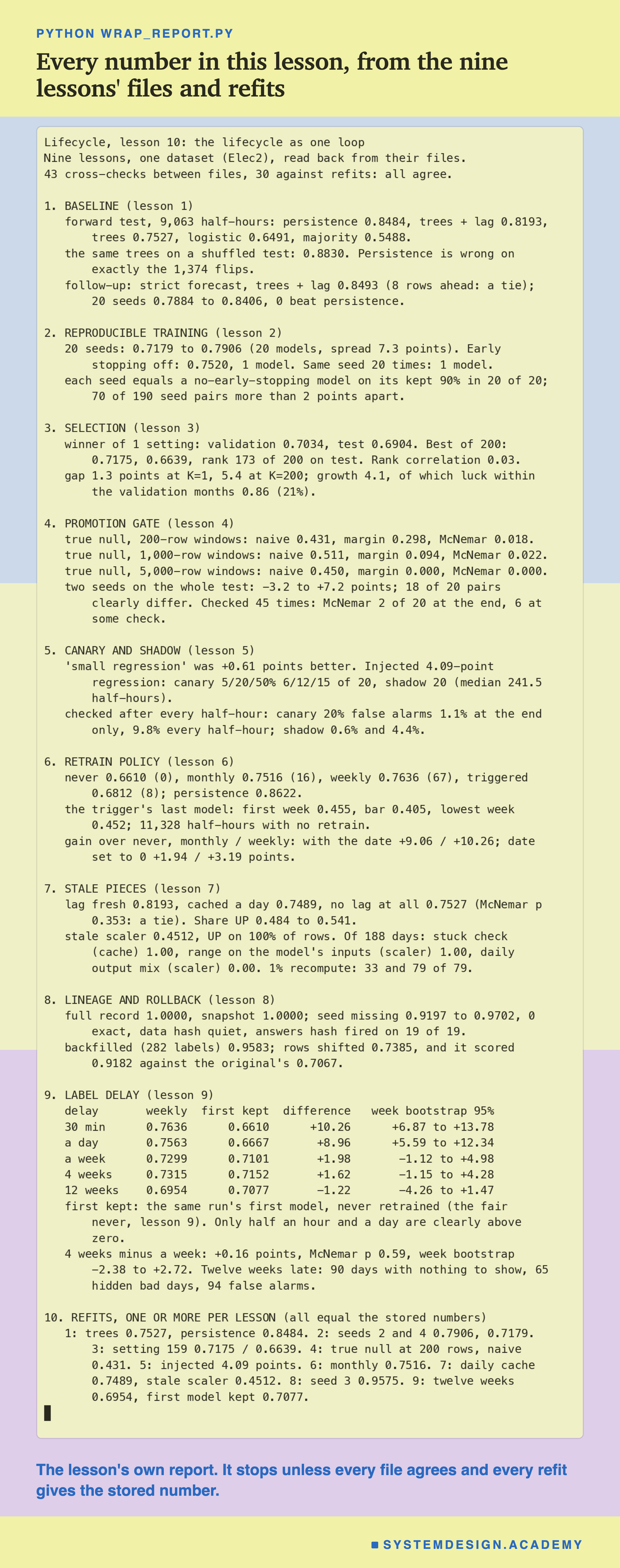
The report lives in scripts/labs/lifecycle/wrap_report.py. It reads the nine labs' stored files and their reports' files, from baseline.json for lesson 1 to delay.json, delay_followup.json and delay_fairnever.json for lesson 9, and it checks them in two ways before it prints anything. Where a lab's file and its lesson's report file both hold a number, they must agree: 43 comparisons. And for every lesson, it trains the lab's models again with the lab's own data, split, settings and seeds and stops unless the stored headline comes back exactly: 30 refit checks, including lesson 4's coin-swap null on 20 pairs of models and lesson 9's weekly retrain with labels twelve weeks late, together with its first model kept. It changes nothing in any lab's files. Its tryit mode, added after this lesson's review, makes the try-it slide's edit on a copy of the demo, runs it, checks the printed agreement against its own refit, and stores the run in .

This box has no model in it. It holds the nine steps, each with what it is for, the failure its lesson measured, what saw it and what the lesson could not show, written from the report's numbers. It runs in your browser.

As it is, the box prints the loop: each step with what it is for and its measured failure, and a last line that sends you back to step 1. The report's box mode checks that every printed failure is the one it built from the stored files.

Try step(8) to see one step in full, with what saw the failure and what the lesson could not show. Try unseen() to list, by my reading and the rule on the matrix slide, the step no check saw at the time and the steps only checks chosen after the results saw: it prints steps 6, 7 and 9. Then describe your own pipeline: gaps(1, 4, 8) lists every step you did not name, each with what this chapter measured there.

Loading. fetch_openml("electricity", version=1) downloads Elec2 once and reads the local copy after that. The label column holds the words UP and DOWN, turned into 1 and 0. cut is 36,249: the first 80% of the rows in time are for learning, the rest are the future.

sha. Feeds the exact bytes of one or more arrays into SHA-256 and keeps the first 12 characters of the fingerprint. np.ascontiguousarray lays the numbers out in one fixed order first, so the same table always gives the same bytes. Twelve characters are enough to compare by eye; a real record keeps all 64.

The baseline. The boosted trees with seed 0 learn from the first 80% and answer the rest. y[cut - 1:-1] == y[cut:] scores persistence: each test row is paired with the label before it. The if prints the verdict, because the check is only useful if someone acts on it.

The fingerprints. The model of lesson 8 learns from rows 0 to 30,000 with seed 7 and answers the next 6,000, the rows it "served". The data hash and the answers hash are the record. The loop rebuilds it twice, with the recorded seed and with a guess, and compares both hashes with the record each time. The data hash is computed from the rows the rebuild learned from; here they are the same rows, so it says "same" both times, which is exactly why it cannot see a lost seed.

The output mix. The logistic model learns behind a scaler fitted on the training rows, then answers through an old scaler fitted on the first 10% of rows, as in lesson 7. The script prints the share of UP answers, which needs no labels, next to the share of UP in the training labels.

The checklist is the what. Here is the how, in the order I would add the checks to a pipeline that has none, cheapest and most often useful first.

Start with the two numbers that cost nothing. Score persistence, or whatever your laziest rule is, on the same future rows as your model, and print the share of each answer the model gives next to the share in its training labels. Both need a few lines and no new data. The first tells you whether the model is worth running at all. Trust the second little: in lesson 9 it moved with weekly accuracy only partly, a rank correlation of about -0.60, so it says where to look, not what is wrong. In the demo the trees said UP on 0.512 of the test rows against 0.418 of the training labels, while 0.451 of the test rows really were UP; a gap like that is a reason to look closer, not proof that anything broke.

Then make every run leave a record. Save the model file, the row numbers or dates it learned from, the seed, every setting and the library versions, and two fingerprints: of the training rows and of the model's answers on a fixed set of rows. Keep it next to the model, by version, in a registry you control, because loading a pickle can run hidden code, and do not count on a file loading under another scikit-learn version, which scikit-learn does not support. From then on, a rollback is a load and a comparison of two hashes.

Then put a paired check in front of every replacement. Keep the champion's answers on your evaluation rows, and compare any challenger on the same rows with McNemar's test, with the rule and the number of rows written down before anyone sees a score. If you can afford it, run the challenger in shadow on live rows before any user sees it.

Then look for stale pieces. List every cache and every saved file the pipeline loads. Store the time each value was computed and the model version each file belongs to, and recompute a small sample fresh every day.

Then measure time. Find out how late your labels really arrive, score a frozen copy of the model block by block, and find the inputs that only say when. Only then choose a retraining schedule, and compare it with the first model kept, not with a model that had labels you will never have.

Last, run the expensive checks when a decision depends on them. Several seeds before you believe a gain, a clean test set before you report a tuned score, a replay of any trigger's log before you trust it.

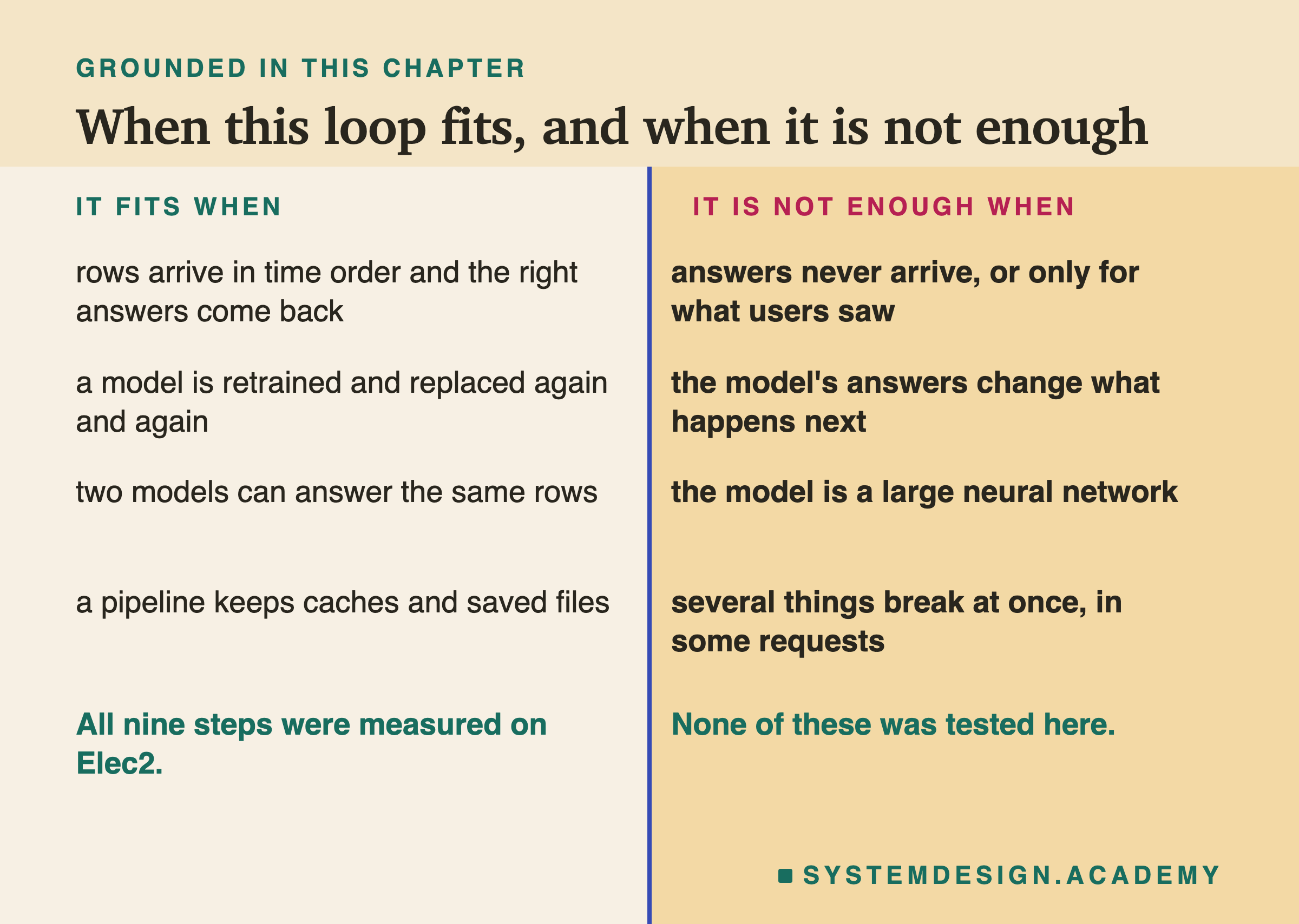
Use this loop when rows arrive in time order and the right answers come back. Prices, demand, sensor readings, whether a server was busy. That is the kind of job this chapter measured, and every step has a number from it.

Use it when a model is retrained and replaced again and again. Steps 2, 4, 6 and 8 are about exactly that: a new model is a different model, and each replacement needs a record, a paired gate and a way back.

Use it when two models can answer the same rows. The two strongest checks in the chapter, McNemar's test at the gate and shadow in rollout, both depend on it.

Use it when a pipeline keeps caches and saved files. Step 7 applies to any stored piece that a later step loads.

It is not enough when the answers never arrive, or arrive only for what users saw. Then accuracy cannot be measured at all, shadow cannot be scored, and steps 5 and 9 change shape. This chapter never tested that.

It is not enough when the model's answers change what happens next. A recommendation changes what people click; the electricity price went up or down whatever the model said. The previous chapter's feedback-loop lesson measured that case, on bikes; this one did not.

It is not enough for large neural networks or language models as they stand. Their randomness, their cost of a retrain and their outputs are different, and none was tested here. The questions carry over; the numbers do not.

It is not enough when several things break at once. Every failure here was one fault at a time, often built on purpose.

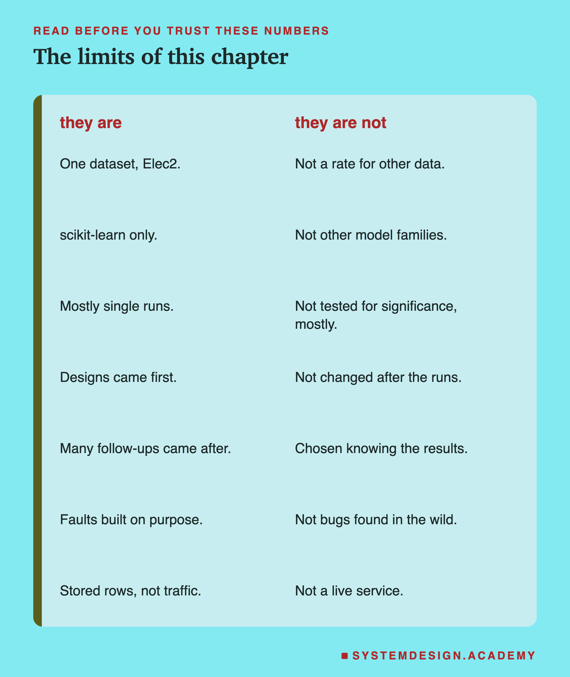
One dataset. Every number in this chapter comes from Elec2, 45,312 half-hours of one electricity market in New South Wales, from May 1996 to December 1998. Its label is sticky by its own definition, a price against a slow 24-hour average, and its date input grows with time. Both shaped several results. On other data the ranking of these failures could be very different, and persistence could be weak.

scikit-learn only. Every model was a scikit-learn model: boosted trees, and logistic regression as a second model. Some findings depend on how boosted trees work, such as a date past the training range falling into the last range the trees saw, and on one default setting, early stopping. Neural networks and language models were never tested.

Single runs, mostly. Most labs ran each setting once. The exceptions were deliberate and small: 20 seeds in lesson 2 and in lesson 1's follow-up, 200 settings and 1,000 draws in lesson 3, 20 seed pairs in lesson 4, 20 starting points that overlap in lesson 5, 19 guessed seeds in lesson 8, and bootstraps in lessons 3 and 9. Few gaps in this chapter were tested for significance, and I have called gaps that could not be told apart from chance exactly that.

Several follow-ups designed after the results. Every lab's design was written before it ran. But lessons 1, 3, 4, 5, 6, 7, 8 and 9 each added a follow-up designed after the main results, and several key numbers come from them: the strict forecast, the fair luck control, the true null, the injected regressions, the date set to 0, the cache intervals, the answers fingerprint's count, and the first model kept. Lesson 2's rebuild of each seed's hidden slice, behind its 20 of 20, was also added after the results. Many of the checks in lesson 7, the levels behind lesson 9's hidden bad days, and the table of which check saw what were chosen knowing the results.

No real production traffic. Live traffic was always stored rows replayed in time order, one row per half-hour. The faults were built on purpose. The lineage "month" was simulated in one process on one machine. No user ever saw an answer.

Take one model your team runs, open the checklist, and answer the nine lines in order. For each one, write down the check you run today, or "nothing". The lines where you write "nothing" are your map with the pins still to come.

Then do the three cheapest things this week. Score persistence, or your own laziest rule, on the same future rows as the model. Print the share of each answer next to the share in the training labels. And add the answers fingerprint to the record of the model you would roll back to, so that the next rebuild, or the next reload, can prove it is the same model. The demo on this lesson's try-it slide runs all three on Elec2.

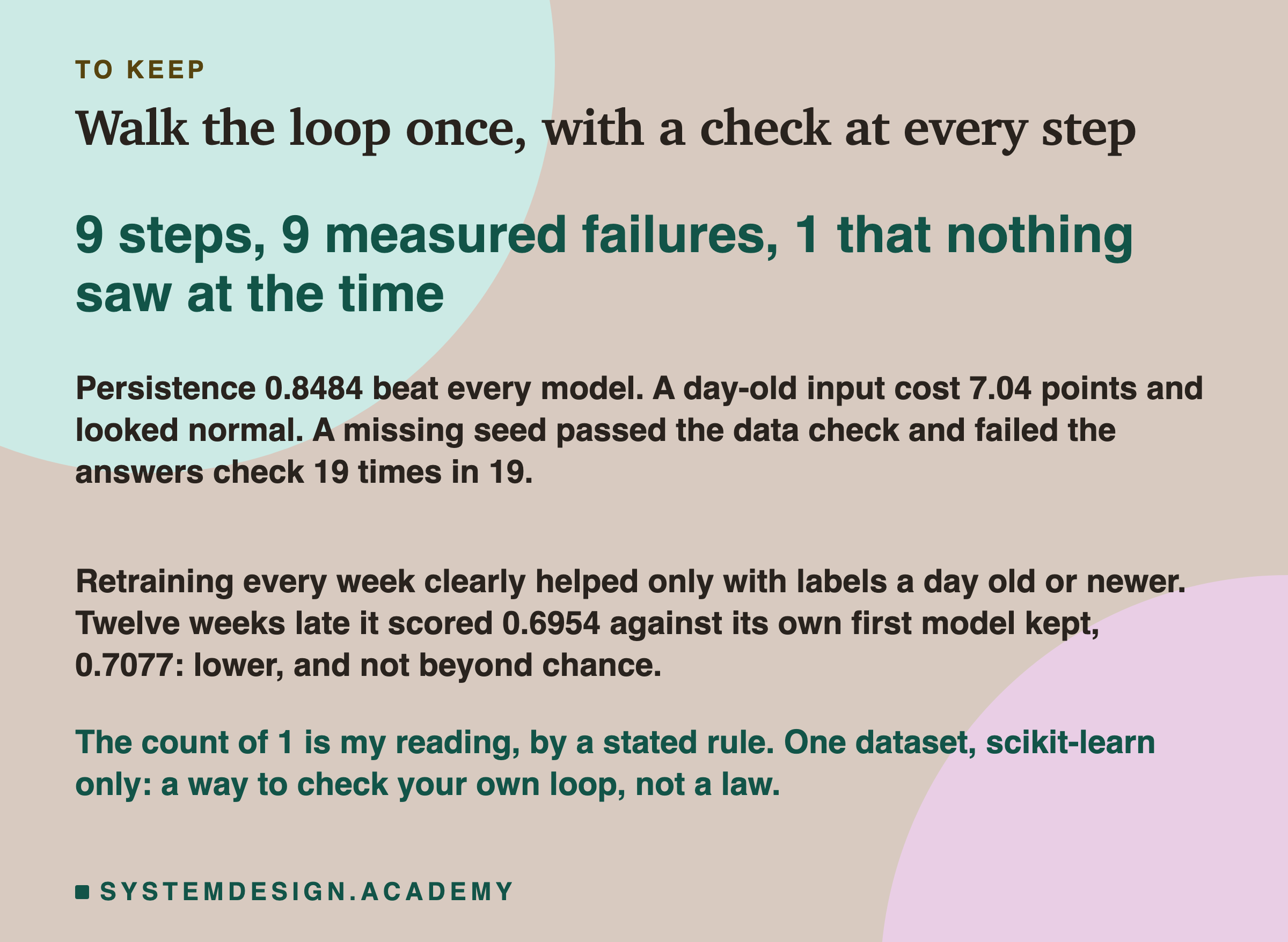
This is the end of the chapter. Each lesson measured one step, and this one put the steps back into a loop. The next chapter planned for the course moves on from the life of one model to the next part of the curriculum, and the checks from this page go with it.